A Structured, Tagged, and Localized Visual Question Answering Dataset with Full Sentence Answers and Scene Graphs for Chest X-Ray Images
Mobile reading edition. English text is reflowed for small screens; original figures and diagrams stay inline, while paper tables are rebuilt as responsive HTML tables.
1 Chair for AI in Healthcare and Medicine, Technical University of Munich (TUM) and TUM University Hospital, Germany 2 Department of Diagnostic and Interventional Radiology, TUM University Hospital, Germany 3 Hasso Plattner Institute for Digital Engineering, University of Potsdam, Germany 4 Department of Computing, Imperial College London, UK 5 Munich Center for Machine Learning (MCML), Germany
ABSTRACT
Visual Question Answering (VQA) enables targeted and context-dependent analysis of medical images, such as chest X-rays (CXRs). However, existing VQA datasets for CXRs are typically constrained by simplistic and brief answer formats, lacking localization annotations (e.g., bounding boxes) and structured tags (e.g., region or radiological finding/disease tags). To address these limitations, we introduce MIMIC-Ext-CXR-QBA (abbr. CXR-QBA), a large-scale CXR VQA dataset derived from MIMIC-CXR, comprising 42 million QA-pairs with multi-granular, multi-part answers, detailed bounding boxes, and structured tags. We automatically generated our VQA dataset from scene graphs (also made available), which we constructed using LLM-based information extraction from radiology reports. After automatic quality assessment, we identified 31M pre-training and 7.5M fine-tuning grade QA-pairs, providing the largest and most sophisticated VQA dataset for CXRs to date. Tools for using our dataset and the construction pipeline are available at https://github.com/philip-mueller/mimic-ext-cxr-qba/.
1 INTRODUCTION
With the emergence of Large Language Models (LLMs) and Large Multimodal Models (LMMs), interactive and conversational tasks have gained popularity in medical image analysis, particularly in the context of chest X-ray (CXR) interpretation (Chen et al., 2024; Müller et al., 2025; Tu et al., 2024; Xie et al., 2025). A prominent example of such interactive tasks is Visual Question Answering (VQA), where a model is presented with an image and a corresponding textual question, and is tasked with generating an answer. Unlike conventional medical imaging approaches, which always produce the same output (such as classification labels, bounding boxes, or textual reports) for a given image, VQA enables users to interactively explore and interpret images in a context-dependent manner. Training robust VQA models for medical applications requires high-quality, large-scale training datasets. Existing CXR VQA datasets suffer from several limitations: (i) they often contain only short and simplistic answers, (ii) they lack localization information (such as bounding boxes), and (iii) they provide little structured metadata (e.g., region and finding/disease annotations, or uncertainty estimates). Additionally, their relatively small size constrains their utility for pretraining.
To address these challenges, we propose a pipeline for automatic VQA dataset creation and apply it to construct a new large-scale CXR VQA dataset. Unlike prior datasets, each question-answer (QA) pair includes multi-granular, multi-part answers composed of full sentences in the style of radiology reports. Furthermore, our dataset provides detailed bounding boxes and additional structured tags (e.g., findings and regions), enhancing interpretability and facilitating the development of more advanced and transparent medical VQA models. Fig. 1 shows examples of our generated QA-pairs.
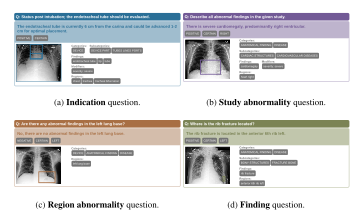
Figure 1: Examples of question-answer (QA) pairs for each of our four different types of questions. For each question (for a given chest X-ray), a detailed answer with sentences in the style of free-text radiology reports is given, supplemented by bounding boxes (for both positive and negative answers), and a set of tags (e.g. regions, findings, certainty, etc.). For more examples, we refer to Sec. A.
Our contributions are as follows:
- We propose an automatic dataset construction pipeline for large-scale medical VQA datasets, offering structured, tagged, and localized answers. To provide a reliable data source for this pipeline, we develop an automatic scene-graph construction method.
- Building on this, we introduce MIMIC-Ext-CXR-QBA (abbr. CXR-QBA), a CXR VQA dataset of 42M question–answer pairs derived from MIMIC-CXR (Johnson et al., 2024b).
- We automatically assess the quality of the generated QA-pairs, identifying 31.2M pairs as pre-training (PT) grade and 7.5M of these as fine-tuning (FT) grade.
- We perform extensive quality controls, including validations against expert annotations and assessment of the automatic ratings, ensuring the robustness of our pipeline.
- We introduce the structured VQA task for CXRs and provide a baseline model to demonstrate our dataset’s utility and guide future model development.
2 RELATED WORK
VQA Datasets for Chest X-Rays VQA datasets (shown in Tab. 1) are scarce in the medical imaging domain, with most notable examples being VQA-RAD (Lau et al., 2018) and SLAKE (Liu et al., 2021), which are hand-labeled but limited in size. On the other hand, VQA-Med at ImageCLEF 2019 (Ben Abacha et al., 2019) was automatically constructed using QA templates based on image annotations, which may limit its answer quality. To improve the quality, PMC-VQA (Zhang et al., 2024) used an LLM to generated QA-pairs based on provided captions. VQA datasets for chest X-rays include MIMIC-Ext-MIMIC-CXR-VQA (Bae et al., 2024) and Medical-CXR-VQA (Hu et al., 2025; 2024), which contain hundreds of thousands of QA-pairs, derived from MIMIC-CXR. These datasets rely on templates but use radiology reports as their original
| Dataset | #QA | Boxes | Tags | Answers |
|---|---|---|---|---|
| CXR-QBA (Ours) | 42.2M | ✓ | ✓ | detailed |
| ↳ fine-tuning grade | 7.5M | |||
| VQA-RAD | 3.5K | ✗ | ✗ | brief |
| SLAKE | 14K | ✗ | ✗ | brief |
| ImageCLEF | 15K | ✗ | ✗ | brief |
| PMC-VQA | 227K | ✗ | ✗ | brief |
| MIMIC-CXR-VQA | 377K | ✗ | ✗ | brief |
| Medical-CXR-VQA | 780K | ✗ | ✗ | brief |
| CheXinstruct | 8.5M | ✗ | ✗ | brief |
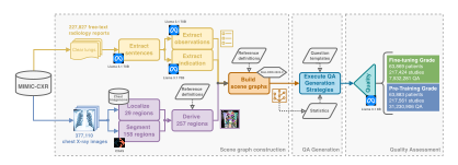
Figure 2: Overview of our dataset construction pipeline. First, we construct scene graphs based on information extracted from the radiology reports and regions localized in the images. Next, we generate question-answer pairs based on templates and the scene graphs. Finally, we automatically assess the quality of generated QA-pairs.
information source, where MIMIC-Ext-MIMIC-CXR-VQA leverages Chest ImaGenome’s (Wu et al., 2021a) scene graphs and Medical-CXR-VQA employs an LLM-based extraction strategy similar to ours but without semantic entity mapping, localization, and extraction of textual descriptions. The largest chest X-ray VQA dataset to date, CheXinstruct (Chen et al., 2024), contains 8.5M QA-pairs with images from multiple data sources. However, compared to our dataset, its questions and answers are less diverse, being purely template-based and derived from dataset annotations instead of being directly conditioned on the reports. Additionally, none of the described datasets provide the level of detail and annotation richness found in our dataset, which includes bounding boxes, tags, and more detailed, multi-part answers that mirror radiology report sentences.
Grounded Report Generation While localization is not yet common for medical VQA tasks, grounded report generation, i.e. predicting radiology reports with bounding boxes is gaining popularity. Notable examples include MAIRA-2 (Bannur et al., 2024), trained on reports manually annotated with bounding boxes and MedTrinity-25M (Xie et al., 2025), a large-scale public dataset with automatically generated reports with bounding boxes. ChEX (Müller et al., 2025) is another model producing textual answers with bounding boxes but does not support VQA tasks.
Scene Graph Construction for Chest X-Rays During our VQA dataset construction, we automatically derive scene graphs from radiology reports. A similar approach is employed by Chest ImaGenome (Wu et al., 2021a;b), which uses rule-based information extraction, and RadGraph (Jain et al., 2021), which uses a relation extraction model. We do not rely on any of those scene graphs but instead leverage LLM-based extraction with semantic entity mapping to extract our own more comprehensive and reliable scene graphs. Notably, our method defines a larger set of (localized) regions (257) and findings (221) compared to Chest ImaGenome (29 regions, 53 findings), while additionally rewriting report sentences to focus on specific aspects related to individual graph nodes.
3 THE CXR-QBA DATASET
We present our dataset CXR-QBA, a large-scale chest X-ray (CXR) VQA dataset derived from MIMIC-CXR (Johnson et al., 2024b; 2019a), consisting of more than 42M QA-pairs. As shown in Fig. 1, each QA sample (for a given chest X-ray) consists of a question (Q), a bounding box (B) supplemented answer (A), and additional tags (regions, findings, certainties, and more). To build our dataset, we propose an automatic pipeline highlighted in Fig. 2. More specifically, we first construct (visually grounded) scene graphs based on the MIMIC-CXR radiology reports using LLM-based information extraction, semantic concept mapping, and localization models (Sec. 3.1). These scene graphs provide a structured description of the study, including sentences (derived from the report) for individual observations. They serve as a data source for our question-answer generation, where we utilize both template-based answers and answers derived from the rewritten report sentences (Sec. 3.2). Finally, we automatically assess the quality of question-answer pairs using LLM-based evaluations (Sec. 3.3).
3.1 SCENE GRAPH CONSTRUCTION
Given a MIMIC-CXR study with a radiology report and accompanying CXRs, we construct a scene graph (Sec. D.1) consisting of sentence nodes, observation nodes, region nodes, an indication node, and edges between them. Sentence nodes are directly extracted from the reports, containing the raw sentences and their identified section names. Observation nodes represent individual aspects described in the report’s FINDINGS or IMPRESSION section, containing (i) a textual description, (ii) bounding boxes for associated CXR images and (iii) additional tags, such as positivity, certainty, laterality, regions, and finding classes. Region nodes are created for mentioned anatomical structures and key regions. The indication node contains information from the INDICATION section, including a textual description and an individual observation node, derived from the FINDINGS and IMPRESSION sections, that can act as an answer to the indication. We construct these scene graphs in three steps: (a) region localization, (b) information extraction and (c) building the graphs using entity mapping. We refer to Sec. E.1 for details.
Region Localization The bounding boxes in our scene graphs (and the derived QA-pairs) are based on fine-grained anatomical structures, allowing us to localize associated findings very precisely. We use the CXAS (Seibold et al., 2022; 2023) model to predict segmentation masks of 158 anatomical structures on the 377 110 CXRs from MIMIC-CXR-JPG (Johnson et al., 2024a; 2019b). Additionally, we use the bounding boxes provided by the Chest ImaGenome (Wu et al., 2021a;b) dataset, which are provided for 29 anatomical structures in most frontal images of MIMIC-CXR. Next, we derive a total of 257 localized anatomical structures based on combinations (e.g. intersections, unions, super bounding boxes, etc.) of the available masks and bounding boxes. Finally, we discard any masks or boxes that are too small and derive bounding boxes from the segmentation masks. Note that we define 53 further regions/structures that are either non-localized (e.g. interstitial) or for which we do not have bounding boxes, leading to a total of 310 structures/regions.
Information Extraction We use the 227 827 free-text radiology reports provided by MIMIC-CXR as the main source of information for our scene graphs. Using the Llama 3.1 70B (Grattafiori et al., 2024) model with few-shot prompting, we extract the relevant information (tags and textual descriptions) in three steps. First, we extract individual sentences from the reports and detect their sections. Next, we extract information about the INDICATION section and detect which FINDINGS or IMPRESSION sentences may provide information related to the indication. Finally, we extract individual observations described in the FINDING/IMPRESSION sentences.
Building Scene Graphs using Entity Mapping Given the extracted information from the reports and the computed bounding boxes, we now construct the final scene graph. Therefore, we first map extracted tags to pre-defined sets of values, our reference definitions. This assures high quality and consistency of the scene graphs and enables mapping of observations to the extracted bounding boxes. The reference definitions are based on tags used in other datasets (including PadChest (Bustos et al., 2020) and Chest ImaGenome (Wu et al., 2021b)) as well as SNOMED-CT (SNOMED International, 2023)) and have been verified by clinical experts. They include synonym lists, hierarchies, and relationships. For more robust mapping, we utilize the BioLORD (Remy et al., 2024) model as a sentence transformer and identify the closest matching concept based on their semantic embeddings. Additionally, we try to fill in missing information where possible, such as inferring the region from an identified finding. Finally, we build a tree of region nodes (using the reference data) and attach the indication information extracted from the report.
3.2 QUESTION-ANSWER GENERATION
Based on the information available in the scene graphs, we generate question-answer pairs (Sec. D.2) using a template-based approach co-designed with radiologists. We incorporate the textual descriptions from the observation nodes – which have been derived directly from the report – to provide diverse and fine-grained answers. Each answer may consist of multiple answer parts (as shown in Fig. 3 and Sec. A), each describing an individual aspect of the answer with its own sentence, bounding boxes, and tags. We categorize answer parts into three types: (i) main-answers, (ii) details, and (iii) related-information, allowing for controlled answer granularity. Answer parts are generated either from templates using scene graph information or directly from observation nodes (Sec. E.2). Answer parts may also be structured hierarchically, where we use parent-child edges from the scene graph.
To generate the question-answer pairs, we employ different strategies for the four types of questions (shown in Fig. 1):
1. Indication: We use the paraphrased indication as the question and create the answer based on the indication node in the scene graph, answering the indication based on information in the FINDINGS and IMPRESSION sections.
2. Study abnormality: We generate study-level questions using 13 different templates, with answer parts (Fig. 3) based on (filtered) observation nodes.
3. Region abnormality: We generate questions about individual regions using 6 different templates, considering any region mentioned and additionally randomly sampling non-mentioned regions for balancing.
4. Finding: We generate questions about individual findings using 7 different templates, considering any finding mentioned and additionally randomly sampling non-mentioned findings for balancing.
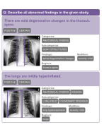
Figure 3: Answer with multiple parts for different aspects, each with a sentence, tags, and boxes.
3.3 QUALITY ASSESSMENT
The dataset construction procedure described so far allows us to automatically generate large amounts of QA-pairs. However, in each of the steps, errors may be introduced, affecting the overall quality of the dataset. For example, errors during information extraction could lead to incorrect tags, therefore leading to incorrectly filled answer templates or incorrectly selected observation nodes for answers.
To identify and filter such cases, we employ an automatic quality assessment strategy using an LLM-as-a-judge. More specifically, we use Llama 3.1 8B (Grattafiori et al., 2024) to rate questions and answers by the following five criteria: entailment (does the answer factually align with the original report?), relevance (is the answer relevant to the question?), completeness (is the answer missing something?), as well as question and answer clarity (is the question/answer clear and grammatically correct?). Additionally, we assess the quality of the used scene graphs by identifying missing information (e.g. missing tags or localization) or issues during the construction process. Finally, we combine these individual assessments into an overall quality rating as one of A++, A+, A, B, C, D, or not rated (Sec. D.3). Based on these ratings, we propose two subsets, one for pre-training and one for fine-tuning. We exclude all non-frontal images from these datasets, as the localization quality on these images is comparatively low due to limitations in the localization models. All QA-pairs with a grade of A or better are labeled as fine-tuning (FT) grade, resulting in 7.5M pairs, while samples with grade B or better are considered pre-training (PT) grade, resulting in 31.2M pairs.
4 EVALUATION AND ANALYSIS
4.1 EVALUATION OF THE SCENE GRAPHS
For the evaluation of the components in our pipeline, we refer to their original publications. The CXAS (Seibold et al., 2022; 2023), used as our primary region localization model, was evaluated against expert annotations on 60 images from PadChest (Bustos et al., 2020). They reported mIoU scores of 0.93 (frontal images) and 0.85 (lateral images), compared to an inter-rater agreement of 0.95 and 0.83, respectively. The BioLORD model (Remy et al., 2024), used for entity mapping, was evaluated on tasks like clinical semantic textual similarity and clinical named entity linking, achieving multi-benchmark average scores of 89.0 (Pearson correlation) and 59.2 (Top-1 accuracy), respectively.
To evaluate the full graph construction pipeline, including the LLM-based extraction, we evaluate our scene graphs by comparing their tags and bounding boxes to hand-labeled expert annotations on MIMIC-CXR. For comparison, we include the scene graphs from Chest ImaGenome (Wu et al., 2021a) as a baseline. First, we evaluate the plausibility of finding tags by comparing study-level
| MIMIC-CXR-JPG Test [MCC] | CXR-LT 2024 Gold [MCC] | ||||||||
|---|---|---|---|---|---|---|---|---|---|
| Classes | CXP-5 | CXP-7 | CXP-13 | Micro | CXP-7 | CXP-13 | LT-only | CXR-LT | Micro |
| Ours (scene graphs) | 0.8[0.77, 0.82] | 0.81[0.79, 0.84] | 0.69[0.67, 0.71] | 0.71[0.69, 0.73] | 0.65[0.61, 0.69] | 0.57[0.54, 0.6] | 0.71[0.67, 0.74] | 0.64[0.61, 0.66] | 0.67[0.65, 0.69] |
| Chest ImaGenome | 0.78[0.75, 0.81] | 0.8[0.78, 0.83] | 0.66[0.64, 0.69] | 0.67[0.65, 0.68] | 0.65[0.61, 0.68] | 0.56[0.54, 0.59] | 0.59[0.55, 0.63] | 0.58[0.55, 0.6] | 0.64[0.62, 0.66] |
| MS-CXR | REFLACX | |||||
|---|---|---|---|---|---|---|
| IoU@30 | IoP@30 | IoT@30 | IoU@30 | IoP@30 | IoT@30 | |
| Ours (scene graphs) | 0.51[0.47, 0.54] | 0.56[0.52, 0.6] | 0.94[0.92, 0.96] | 0.45[0.44, 0.47] | 0.54[0.53, 0.56] | 0.87[0.86, 0.88] |
| Chest ImaGenome | 0.45[0.42, 0.49] | 0.48[0.45, 0.52] | 0.98[0.97, 0.99] | 0.42[0.4, 0.43] | 0.46[0.44, 0.47] | 0.95[0.94, 0.96] |
labels derived from our scene graphs to two reference annotation sets: the radiologist annotations in MIMIC-CXR-JPG v.2.1.0 (Johnson et al., 2024a) with 13 CheXpert (Irvin et al., 2019) classes and the CXR-LT 2024 (Holste et al., 2025; 2024) gold-standard dataset (task 2 test set) with 12 additional rare (long-tail) classes. As shown in Tab. 2a, our approach (slightly) outperforms Chest ImaGenome, with strong improvements (20%) on long-tail classes, demonstrating the value of our fine-grained finding tags (221 classes) in capturing nuanced study details. Further results are provided in Sec. C.2.
To evaluate the accuracy of finding bounding boxes, we compare them with annotations from MS-CXR (Boecking et al., 2024; 2022) (6 classes) and REFLACX (Bigolin Lanfredi et al., 2021; 2022) (18 classes). We compute study-level pixel masks for each finding as the union of all bounding boxes from positive observation nodes that contain the specific finding tag. We calculate pixel-level Intersection-over-Union (IoU), Intersection-over-Prediction (IoP), and Intersection-over-Target (IoT) for each finding class, considering only image pairs with positive predictions and targets. Thresholding at 30% IoU/IoP/IoT, we micro-average the results, reporting the percentage of accurately localized finding-boxes in Tab. 2b. On the IoU metric, our scene graphs perform slightly better than the ones from Chest ImaGenome. The low IoP values indicate that boxes are often too large, but high IoT values suggest that they generally cover the finding boxes well. This discrepancy arises because boxes are derived from anatomical regions mentioned in reports, whereas hand-labeled annotations are more precise. Notably, our approach produces more precise boxes (higher IoP) than Chest ImaGenome, likely due to our large number of fine-grained region annotations (257 region classes).
Our analysis confirms that our scene graphs contain plausible finding tags and bounding boxes, with competitive or better quality than Chest ImaGenome. The bounding box quality, in turn, validates the plausibility of our region tags. Overall, our construction process yields high-quality scene graphs, making them a reliable foundation for generating QA samples.
4.2 QUALITY OF THE QA-SAMPLES
We assess the quality of our 42.2M QA pairs using an LLM-as-a-judge approach co-designed with trained radiologists (Sec. 3.3). For quality control, we conducted a human study across the five rating
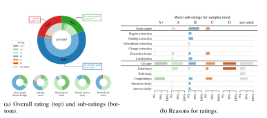
Figure 4: Results of quality assessment (Sec. 3.3). We identified a significant amount of fine-tuning grade samples, while even pre-training grade samples provide factually accurate answers, especially having high quality main answers.
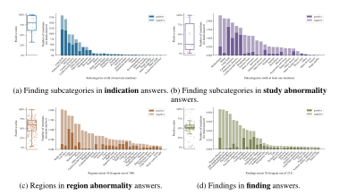
Figure 5: Distribution of tags (finding subcategories, regions, findings) mentioned in answers of different question types (indication, study abnormality, region abnormality, finding). We show their positive ratios, i.e. how often they are mentioned in positive versus in negative answers (left) and plot the number of positive and negative mentions of the most frequent tags (right). These fine-grained tags enable filtering and balancing the dataset or can be used as additional supervision.
criteria (entailment, relevance, completeness, question clarity, and answer clarity), sampling 100 cases per criterion and rating them with the same information provided to the LLM. We found that at most 2% of cases were overrated by the LLM (e.g., assigning fine-tuning instead of pre-training grade), with high overall agreement (Cohen’s kappa) and a slight tendency of the LLM to be more critical than human ratings (Sec. C.1). Quality rating results for our dataset are shown in Fig. 4a. We found that 18.6% were fine-tuning grade, 58.8% were pre-training grade, and 22.6% were marked for exclusion. Notably, 85% of individual main answers were rated A or higher. We also analyzed the main causes of ratings (Fig. 4b) and found that A+ samples were limited by minor incompleteness (minor details missing), A samples by minor entailment aspects (facts not explicitly mentioned in the report), while B samples were restricted by issues with region/finding/localization extraction, completeness, and text clarity. Ratings C were caused by major incompleteness or extraction issues, ratings D by contradicting entailments, while non-rated samples where due to the LLM-judge not producing parsable outputs. Our analysis shows that even pre-training grade samples provide factually accurate answers with minor flaws, making them suitable for pre-training purposes.
4.3 FINDING- AND REGION-DISTRIBUTION IN QA-SAMPLES
Our answers include additional tags for findings (and their categories), regions, and answer positivity (positive or negative finding), enabling filtering and balancing for specific applications. For instance, undersampling negative answers can help mitigate model biases towards negative predictions. In Fig. 5 we analyze the distribution of these tags. We observe that indication questions tend to have more positive mentions (Fig. 5a) – as there is a specific indication to check for – while study abnormality questions have more negative ones (Fig. 5b) – as many samples are negative overall. In region abnormality questions, most regions are mentioned slightly more often with positive than with negative findings (Fig. 5c), while for finding questions mentions are mostly balanced (Fig. 5d). This shows the success of our balanced region/finding sampling used for these two question types.
4.4 UNIQUENESS OF QA-SAMPLES
To measure the effect of our template-based QA generation strategy on the duplication of QA pairs, we count the numbers of (i) unique question texts, (ii) unique answer texts, (iii) unique finding tag sets in answers, and (iv) unique region tag sets in answers. We compare these to the overall number of QA samples to compute the average duplication factor. Results are shown in Tab. 3. As expected, we have high duplication rates for question texts except for indication questions, where the questions are based on the indication section of each report, leading to many unique questions. Despite the template-based questions, we still provide thousands of different individual questions. More notable is the low duplication rate of answer texts, ranging from 1 to 6 for different answer types. This is possible, because answer texts are not solely template-based but also include rewrit-ten sentences from the original reports. Overall this demonstrates that we provide a large-scale dataset with diverse answers.
| # Unique Samples | Average Duplications | |
|---|---|---|
| Question Texts | 177 072 | 238 |
| ↳ Indication | 172 452 | ≈ 1 |
| ↳ Study abnormality | 65 | 183 314 |
| ↳ Region abnormality | 3 926 | 5 252 |
| ↳ Finding | 630 | 14 950 |
| Answer Texts | 7 835 760 | 5 |
| Finding Tag Sets | 764 022 | 55 |
| Region Tag Sets | 586 847 | 72 |
4.5 ANSWER CHARACTERISTICS
Our QA-samples provide detailed free-text answers consisting of one or even multiple sentences (i.e. answer parts). In Fig. 6, we analyze the distribution of lengths of these answers and study differences between types of answers or questions. The median answer length is 14 words, with similar lengths for most question types except for indication questions, where answers are much longer (46 words). We also observe that related information answers are much longer (22 words) than main answers (9 words) or details answers (7 words), which is expected as they can provide a lot additional context to the answers. Answers describing positive findings are typically very long (18 words), considerably longer than negative finding answers (10 words). This highlights that our dataset provides nuanced finding description in their answers, following the level of detail typically present in radiology reports.
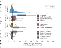
Figure 6: Distribution of answer lengths. We provide nuanced answers with detailed free-text finding descriptions.
| Ours | Baselines | |||||||
|---|---|---|---|---|---|---|---|---|
| Group | Metric | PT(1M) | PT(2M) | FT(1M) | PT(1M)→FT(1M) | MAIRA-2 | Qwen3-VL (4B) | LLaVA-Med v1.5 |
| RadFact | Logical Prec. | 0.67[0.66, 0.68] | 0.68[0.67, 0.69] | 0.76[0.75, 0.76] | 0.78[0.77, 0.78] | 0.25[0.25, 0.26] | 0.63[0.63, 0.64] | 0.47[0.46, 0.48] |
| RadFact | Logical Rec. | 0.69[0.68, 0.69] | 0.70[0.69, 0.70] | 0.75[0.74, 0.76] | 0.77[0.76, 0.77] | 0.64[0.63, 0.65] | 0.58[0.57, 0.59] | 0.08[0.07, 0.08] |
| RadStrucVQA | Grounding Prec. | 0.87[0.86, 0.87] | 0.88[0.87, 0.88] | 0.87[0.87, 0.88] | 0.89[0.88, 0.89] | 0.69[0.67, 0.71] | 0.61[0.60, 0.62] | – |
| RadStrucVQA | Grounding Rec. | 0.92[0.92, 0.93] | 0.92[0.91, 0.92] | 0.89[0.88, 0.89] | 0.90[0.89, 0.90] | 0.12[0.11, 0.12] | 0.51[0.50, 0.52] | – |
| Tags | Finding Prec. | 0.67[0.66, 0.68] | 0.68[0.68, 0.69] | 0.68[0.67, 0.69] | 0.70[0.70, 0.71] | – | – | – |
| Tags | Finding Rec. | 0.61[0.60,0.62] | 0.62[0.61, 0.63] | 0.66[0.66, 0.67] | 0.68[0.68, 0.69] | – | – | – |
| Tags | Finding-pos Prec. | 0.32[0.31, 0.34] | 0.37[0.35, 0.38] | 0.41[0.40, 0.43] | 0.45[0.43, 0.46] | – | – | – |
| Tags | Finding-pos Rec. | 0.13[0.12, 0.14] | 0.16[0.15, 0.17] | 0.26[0.25, 0.27] | 0.31[0.30, 0.32] | – | – | – |
| Tags | Region Prec. | 0.61[0.60, 0.61] | 0.61[0.61, 0.62] | 0.67[0.66, 0.68] | 0.69[0.69, 0.70] | – | – | – |
| Tags | Region Rec. | 0.62[0.61, 0.63] | 0.63[0.62, 0.63] | 0.66[0.65, 0.67] | 0.68[0.67, 0.69] | – | – | – |
5 STRUCTURED VQA TASK
To showcase the utility of our dataset, we introduce the Structured Visual Question Answering (structured VQA) task. Given a free-text question, the model is expected to generate a (multi-part) free-text answer accompanied by bounding boxes and tags (e.g., findings, regions). Unlike classical VQA, this task demands more structured answers, thus improving interpretability and clinical utility.
Baseline Models We implement our own model based on the Llava architecture (Liu et al., 2023), using Rad-DINO (Pérez-Garcı́a et al., 2025) for image encoding and the Llama 3.2 3B (Grattafiori et al., 2024) language model. Our CXR-QBA dataset provides the necessary targets, which we format into sequences using XML-style structures and special tokens to represent tags and bounding boxes. We train this model for one epoch on 1M or 2M pre-training (PT) grade, on 1M fine-tuning (FT) grade, or on 1M pre-training (PT) followed by 1M fine-tuning (FT) grade QA-pairs (MIMIC-CXR train split) and evaluate them on the FT grade test set. For comparison, we include MAIRA-2 (Bannur et al., 2024), the only publicly available CXR report generation model that explicitly supports bounding box prediction. To partially support the task, we adapt its prompt. Furthermore, we include two other vision-language models, namely Qwen3-VL (4b, Instruct) Bai et al. (2025); Team (2025), and LLaVA-Med v1.5 Li et al. (2023), both comparable or larger in size than our model. These models where trained, among others, on VQA instructions. While they were not optimized for bounding box prediction, we still prompt them to provide textual bounding boxes in their answers. They do, however, not support tag prediction. Note that none of the three comparison models was fine-tuned on our task. Additional ablations are provided in Sec. F.1 and further details in Sec. F.3.
RadStrucVQA Metric For evaluation, we introduce the RadStrucVQA metric, which closely follows the RadFact (Bannur et al., 2024) metric introduced for radiology report generation but is generalized to structured VQA. Like RadFact, we identify whether individual predicted answer parts are entailed with target answer parts and vice-versa, in our case using Llama 3.1 8B. For entailed pairs, we compute whether they are visually grounded, i.e. whether their bounding boxes are precise enough considering their references, and whether finding and region tags are correctly reported. This is conducted bi-directionally, using either the targets as references for the predictions or vice-versa, resulting in precision or recall scores, respectively. To verify the reliability of the Llama 3.1 8B model for entailment prediction in our metric, we compared it with Llama 3.1 70B and Qwen3-32B. For all sub-metrics, we found high correlations (0.88 to 0.97) between the small Llama 3.1 8B and the larger models (which almost perfectly agree with each other). More details on the metric and this assessment can be found in Sec. F.2.
Results Results are shown in Tab. 4. Our models achieve high scores in both textual content (logical) and grounding metrics. On most metrics, models trained on the FT grade set outperform models trained only on the PT grade set. Training first on 1M PT samples followed by training on 1M FT samples achieves the best performance, even better than training on 2M PT samples, showing that even our PT grade dataset provides high-quality targets. All of our models outperform the baselines not trained on this task. MAIRA-2 still achieves 75% of our best model’s logical recall, suggesting it captures most relevant information while not contradicting with our answers. However it predicts additional findings (lower precision), probably because it was trained for reporting and cannot react well to questions. MAIRA-2’s grounding precision significantly exceeded its recall, because it was trained to predict bounding boxes only for positive findings. Qwen3-VL outperforms MAIRA-2 on the precision scores indicating that it can better react to questions. Notably, it is almost on-par or outperforms MAIRA-2 in grounding quality. LLaVA-Med v1.5 does not perform well and did not provide bounding boxes (despite being instructed to do so). We assume that this is because that model typically requires fine-tuning on specific tasks and it does not perform well in zero-shot settings. Also, it did not provide individual answers per finding, explaining its low recall. Our models successfully predict finding and region tags in most cases. However, performance drops when focusing solely on positive findings (finding-pos), indicating potential underprediction due to our training procedure or limitations in the pre-trained components. While further analysis would be required, such problems may also lead to flaws in textual answers. Importantly, our dataset’s detailed tags enable fine-grained analysis of such issues while also enabling potential solutions like data filtering or balancing, making it well-suited for complex training scenarios.
6 DISCUSSION
6.1 USE CASES AND IMPACT
We introduced the CXR-QBA dataset, a large-scale, automatically constructed VQA dataset for CXRs offering structured, tagged, and localized answers. By design, it is particularly well-suited for the structured VQA task proposed in Sec. 5. Additionally, its large size and detailed answers make it a valuable resource for pre-training vision-language models. The accompanying tags further enable filtering and balancing of the dataset to suite specific needs. Furthermore, our fine-grained scene graphs with bounding boxes, textual descriptions, and tags can serve as a versatile data source for various purposes. For instance, they can be leveraged to create customized datasets for grounded report generation or VQA, or even as a direct training source for graph generation models to predict scene graphs on unseen chest X-rays, enabling the creation of even larger datasets. Moreover, the bounding boxes and tags provided with the scene graphs can be used for longitudinal analysis, including region-level examination. They can also be used to train models for pathology localization or classification, providing fine-grained and long-tail diagnosis targets that are often lacking in existing datasets. Finally, we release all source code for dataset construction, enabling future work to transfer our dataset construction framework to other modalities beyond chest X-rays.
6.2 LIMITATIONS
Our dataset was automatically constructed, relying on models and templates instead of human annotations. While this enables the generation of a large number of QA-pairs, it may also introduce potential errors and biases like LLM hallucinations or template priors. We apply automatic quality assessments and extensive quality controls to mitigate these risks, but even those have their limitations and some are LLM-based. Therefore, users should be aware that inaccuracies may remain and exercise caution in critical applications. We strongly advise against using this dataset as the sole source for fine-tuning or evaluating models in clinical practice. For such purposes, we recommend using small-scale, gold-standard (fully human-annotated) datasets, which are, however, beyond the scope of this work. Furthermore, our template-based approach may also limit diversity and introduce grammatical errors, though we partially mitigate these issues by incorporating answers from actual report sentences and through quality assessment. Additionally, the dataset is derived from a single source dataset, inheriting demographic and clinical biases present in this specific patient population. This may limit the generalizability of models trained on this dataset. Finally, it focuses on chest X-ray studies from a single dataset, excluding longitudinal and differential questions as well as other imaging modalities. Future work could extend our approach to broader question types and modalities.
ETHICS STATEMENT
This work does not directly involve human subjects and does not collect new human subject data. All human subject data used (such as chest X-rays or radiology reports) are derived from existing public datasets, which were collected independently of and prior to this work. We will release the dataset as a credentialed dataset on the Physionet platform (Goldberger et al., 2000). This ensures compliance with the license of MIMIC-CXR (Johnson et al., 2024b), from which our dataset is derived. It also serves to protect the included data, which is indirectly derived from patient health information. While enabling researcher access, it restricts use for other purposes and requires completion of a privacy and ethics course. Furthermore, to protect privacy and comply with the MIMIC-CXR license, all data processing was performed locally, and no data were sent to external services.
REPRODUCIBILITY STATEMENT
We provide full details to ensure reproducibility of our work. The construction of the dataset is described in Sec. 3, with additional information in Secs. D and E. The structured VQA task and associated metrics are presented in Sec. 5, with further details in Sec. F. All source code for dataset construction and the structured VQA task is available at https://github.com/philip-mueller/mimic-ext-cxr-qba/. The constructed dataset is available through the PhysioNet platform (Goldberger et al., 2000) at https://physionet.org/content/mimic-ext-cxr-qba/1.0.0/. It is accessible to researchers after credentialing by PhysioNet (which requires a short online training). This hosting is necessary because the dataset is derived from MIMIC-CXR.
ACKNOWLEDGMENTS
This work was partially funded by ERC Grant Deep4MI (Grant No. 884622).
REFERENCES
Seongsu Bae, Daeun Kyung, Jaehee Ryu, Eunbyeol Cho, Gyubok Lee, Sunjun Kweon, Jungwoo Oh, Lei JI, Eric Chang, Tackeun Kim, and Edward Choi. MIMIC-Ext-MIMIC-CXR-VQA: A Complex, Diverse, And Large-Scale Visual Question Answering Dataset for Chest X-ray Images, 2024. URL https://physionet.org/content/mimic-ext-mimic-cxr-vqa/1.0.0/.
Shuai Bai, Keqin Chen, Xuejing Liu, Jialin Wang, Wenbin Ge, Sibo Song, Kai Dang, Peng Wang, Shijie Wang, Jun Tang, Humen Zhong, Yuanzhi Zhu, Mingkun Yang, Zhaohai Li, Jianqiang Wan, Pengfei Wang, Wei Ding, Zheren Fu, Yiheng Xu, Jiabo Ye, Xi Zhang, Tianbao Xie, Zesen Cheng, Hang Zhang, Zhibo Yang, Haiyang Xu, and Junyang Lin. Qwen2.5-vl technical report. arXiv preprint arXiv:2502.13923, 2025.
Shruthi Bannur, Kenza Bouzid, Daniel C. Castro, Anton Schwaighofer, Anja Thieme, Sam Bond-Taylor, Maximilian Ilse, Fernando Pérez-Garcı́a, Valentina Salvatelli, Harshita Sharma, Felix Meissen, Mercy Ranjit, Shaury Srivastav, Julia Gong, Noel C. F. Codella, Fabian Falck, Ozan Oktay, Matthew P. Lungren, Maria Teodora Wetscherek, Javier Alvarez-Valle, and Stephanie L. Hyland. MAIRA-2: Grounded Radiology Report Generation, September 2024. URL http: //arxiv.org/abs/2406.04449. arXiv:2406.04449 [cs].
Asma Ben Abacha, Sadid A. Hasan, Vivek V. Datla, Dina Demner-Fushman, and Henning Müller. VQA-Med: overview of the medical visual question answering task at ImageCLEF 2019. Proceedings of CLEF (Conference and Labs of the Evaluation Forum) 2019 Working Notes, September 2019. Meeting Name: CLEF (Conference and Labs of the Evaluation Forum) 2019 Working Num Pages: 11 Place: Lugano, Switzerland Publisher: 9-12 September 2019.
Ricardo Bigolin Lanfredi, Mingyuan Zhang, William Auffermann, Jessica Chan, Phuong-Anh Duong, Vivek Srikumar, Trafton Drew, Joyce Schroeder, and Tolga Tasdizen. REFLACX: Reports and eye-tracking data for localization of abnormalities in chest x-rays, 2021. URL https: //physionet.org/content/reflacx-xray-localization/1.0.0/.
Ricardo Bigolin Lanfredi, Mingyuan Zhang, William F. Auffermann, Jessica Chan, Phuong-Anh T. Duong, Vivek Srikumar, Trafton Drew, Joyce D. Schroeder, and Tolga Tasdizen. REFLACX, a dataset of reports and eye-tracking data for localization of abnormalities in chest x-rays. Sci
Data, 9(1):350, June 2022. ISSN 2052-4463. doi: 10.1038/s41597-022-01441-z. URL https: //www.nature.com/articles/s41597-022-01441-z.
Benedikt Boecking, Naoto Usuyama, Shruthi Bannur, Stephanie Hyland, Maria Wetscherek, Tristan Naumann, Hoifung Poon, and Ozan Oktay. Making the Most of cal Vision–Language Processing. In Shai Avidan, vanni Maria Farinella, and Tal Hassner (eds.), Computer pp. 1–21. Springer Nature Switzerland, Cham, 2022. URL https://link.springer.com/10.1007/978-3-031-20059-5_1. tle: Lecture Notes in Computer Science.
Daniel C. Castro, Anton Schwaighofer, Aditya Nori, Javier Alvarez-Valle, Text Semantics to Improve Biomedi-Gabriel Brostow, Moustapha Cissé, Gio-Vision – ECCV 2022, volume 13696, doi: 10.1007/978-3-031-20059-5 1. Series Ti-
Benedikt Boecking, Naoto Usuyama, Shruthi Bannur, Daniel Coelho de Castro, Anton Schwaighofer, Stephanie Hyland, Harshita Sharma, Maria Teodora Wetscherek, Tristan Naumann, Aditya Nori, Javier Alvarez Valle, Hoifung Poon, and Ozan Oktay. MS-CXR: Making the Most of Text Semantics to Improve Biomedical Vision-Language Processing, 2024. URL https: //physionet.org/content/ms-cxr/1.1.0/.
Aurelia Bustos, Antonio Pertusa, Jose-Maria Salinas, and Maria de la Iglesia-Vayá. PadChest: A large chest x-ray image dataset with multi-label annotated reports. Medical Image Analysis, 66: 101797, December 2020. ISSN 1361-8415. doi: 10.1016/j.media.2020.101797. URL https: //www.sciencedirect.com/science/article/pii/S1361841520301614.
Zhihong Chen, Maya Varma, Justin Xu, Magdalini Paschali, Dave Van Veen, Andrew Johnston, Alaa Youssef, Louis Blankemeier, Christian Bluethgen, Stephan Altmayer, Jeya Maria Jose Valanarasu, Mohamed Siddig Eltayeb Muneer, Eduardo Pontes Reis, Joseph Paul Cohen, Cameron Olsen, Tanishq Mathew Abraham, Emily B. Tsai, Christopher F. Beaulieu, Jenia Jitsev, Sergios Gatidis, Jean-Benoit Delbrouck, Akshay S. Chaudhari, and Curtis P. Langlotz. A Vision-Language Foundation Model to Enhance Efficiency of Chest X-ray Interpretation, December 2024. URL http://arxiv.org/abs/2401.12208. arXiv:2401.12208 [cs].
Ary L. Goldberger, Luis A. N. Amaral, Leon Glass, Jeffrey M. Hausdorff, Plamen Ch. Ivanov, Roger G. Mark, Joseph E. Mietus, George B. Moody, Chung-Kang Peng, and H. Eugene Stanley. PhysioBank, PhysioToolkit, and PhysioNet. Circulation, 101(23):e215–e220, June 2000. doi: 10.1161/01.CIR.101.23.e215. URL https://www.ahajournals.org/doi/full/10. 1161/01.cir.101.23.e215. Publisher: American Heart Association.
Aaron Grattafiori, Abhimanyu Dubey, Abhinav Jauhri, Abhinav Pandey, Abhishek Kadian, et al. The Llama 3 Herd of Models, November 2024. URL http://arxiv.org/abs/2407.21783. arXiv:2407.21783 [cs].
Gregory Holste, Yiliang Zhou, Song Wang, Ajay Jaiswal, Mingquan Lin, Sherry Zhuge, Yuzhe Yang, Dongkyun Kim, Trong-Hieu Nguyen-Mau, Minh-Triet Tran, Jaehyup Jeong, Wongi Park, Jongbin Ryu, Feng Hong, Arsh Verma, Yosuke Yamagishi, Changhyun Kim, Hyeryeong Seo, Myungjoo Kang, Leo Anthony Celi, Zhiyong Lu, Ronald M. Summers, George Shih, Zhangyang Wang, and Yifan Peng. Towards long-tailed, multi-label disease classification from chest X-ray: Overview of the CXR-LT challenge. Medical Image Analysis, 97:103224, October 2024. ISSN 1361-8415. doi: 10.1016/j.media.2024.103224. URL https://www.sciencedirect. com/science/article/pii/S136184152400149X.
Gregory Holste, Mingquan Lin, Song Wang, Yiliang Zhou, Yishu Wei, Hao Chen, Atlas Wang, and Yifan Peng. CXR-LT: Multi-Label Long-Tailed Classification on Chest X-Rays, 2025. URL https://physionet.org/content/cxr-lt-iccv-workshop-cvamd/2.0.0/.
Edward J. Hu, Yelong Shen, Phillip Wallis, Zeyuan Allen-Zhu, Yuanzhi Li, Shean Wang, Lu Wang, and Weizhu Chen. LoRA: Low-Rank Adaptation of Large Language Models. October 2021. URL https://openreview.net/forum?id=nZeVKeeFYf9.
Xinyue Hu, Lin Gu, Kazuma Kobayashi, Liangchen Liu, Mengliang Zhang, Tatsuya Harada, Ronald M. Summers, and Yingying Zhu. Interpretable medical image Visual Question Answering via multi-modal relationship graph learning. Medical Image Analysis, 97:103279, October 2024. ISSN 1361-8415. doi: 10.1016/j.media.2024.103279. URL https://www.sciencedirect. com/science/article/pii/S1361841524002044.
Xinyue Hu, Lin Gu, Kazuma Kobayashi, liangchen liu, Mengliang Zhang, Tatsuya Harada, Ronald Summers, and Yingying Zhu. Medical-CXR-VQA dataset: A Large-Scale LLM-Enhanced Medical Dataset for Visual Question Answering on Chest X-Ray Images, 2025. URL https: //physionet.org/content/medical-cxr-vqa-dataset/1.0.0/.
Jeremy Irvin, Pranav Rajpurkar, Michael Ko, Yifan Yu, Silviana Ciurea-Ilcus, Chris Chute, Henrik Marklund, Behzad Haghgoo, Robyn Ball, Katie Shpanskaya, Jayne Seekins, David A. Mong, Safwan S. Halabi, Jesse K. Sandberg, Ricky Jones, David B. Larson, Curtis P. Langlotz, Bhavik N. Patel, Matthew P. Lungren, and Andrew Y. Ng. CheXpert: A Large Chest Radiograph Dataset with Uncertainty Labels and Expert Comparison. Proceedings of the AAAI Conference on Artificial Intelligence, 33(01):590–597, July 2019. ISSN 2374-3468. doi: 10.1609/aaai.v33i01.3301590. URL https://ojs.aaai.org/index.php/AAAI/article/view/3834. Number: 01.
Saahil Jain, Ashwin Agrawal, Adriel Saporta, Steven Duong, Tan Bui, Pierre Chambon, Yuhao Zhang, Curtis Langlotz, and Pranav Rajpurkar. RadGraph: Relations from Radiology Reports. Proceedings cessing Systems Track on Datasets and Benchmarks, https://datasets-benchmarks-proceedings.neurips.cc/paper/2021/hash/c8ffe9a587b126f152ed3d89a146b445-Abstract-round1.html.
Truong, Du Nguyen Duong N. Matthew Lungren, Andrew Ng, Extracting Clinical Entities and of the Neural Information Pro- 1, December 2021. URL
Alistair Johnson, Matthew Lungren, Yifan Peng, Zhiyong Lu, Roger Mark, Seth Berkowitz, and Steven Horng. MIMIC-CXR-JPG - chest radiographs with structured labels, 2024a. URL https: //physionet.org/content/mimic-cxr-jpg/2.1.0/.
Alistair Johnson, Tom Pollard, Roger Mark, Seth Berkowitz, and Steven Horng. MIMIC-CXR Database, 2024b. URL https://physionet.org/content/mimic-cxr/2.1.0/.
Alistair E. W. Johnson, Tom J. Pollard, Seth J. Berkowitz, Nathaniel R. Greenbaum, Matthew P. Lungren, Chih-ying Deng, Roger G. Mark, and Steven Horng. MIMIC-CXR, a de-identified publicly available database of chest radiographs with free-text reports. Sci Data, 6(1):317, December 2019a. ISSN 2052-4463. doi: 10.1038/s41597-019-0322-0. URL https://www.nature. com/articles/s41597-019-0322-0.
Alistair E. W. Johnson, Tom J. Pollard, Nathaniel R. Greenbaum, Matthew P. Lungren, Chih-ying Deng, Yifan Peng, Zhiyong Lu, Roger G. Mark, Seth J. Berkowitz, and Steven Horng. MIMIC-CXR-JPG, a large publicly available database of labeled chest radiographs, November 2019b. URL http://arxiv.org/abs/1901.07042. arXiv:1901.07042 [cs].
Woosuk Kwon, Zhuohan Li, Siyuan Zhuang, Ying Sheng, Lianmin Zheng, Cody Hao Yu, Joseph Gonzalez, Hao Zhang, and Ion Stoica. Efficient Memory Management for Large Language Model Serving with PagedAttention. In Proceedings of the 29th Symposium on Operating Systems Principles, SOSP ’23, pp. 611–626, New York, NY, USA, October 2023. Association for Computing Machinery. ISBN 979-8-4007-0229-7. doi: 10.1145/3600006.3613165. URL https://dl.acm.org/doi/10.1145/3600006.3613165.
Jason J. Lau, Soumya Gayen, Asma Ben Abacha, and Dina Demner-Fushman. A dataset of clinically generated visual questions and answers about radiology images. Sci Data, 5(1):180251, November 2018. ISSN 2052-4463. doi: 10.1038/sdata.2018.251. URL https://www.nature.com/articles/sdata2018251.
Chunyuan Li, Cliff Wong, Sheng Zhang, Naoto Usuyama, Haotian Liu, Jianwei Yang, Tristan Naumann, Hoifung Poon, and Jianfeng Gao. LLaVA-Med: Training a Large Language-and-Vision Assistant for Biomedicine in One Day. In NIPS ’23: Proceedings of the 37th International Conference on Neural Information Processing Systems, 2023.
Ji Lin, Jiaming Tang, Haotian Tang, Shang Yang, Wei-Ming Chen, Wei-Chen Wang, Guangxuan Xiao, Xingyu Dang, Chuang Gan, and Song Han. AWQ: Activation-aware Weight Quantization for On-Device LLM Compression and Acceleration. Proceedings of Machine Learning and Systems, 6: 87–100, May 2024. URL https://proceedings.mlsys.org/paper_files/paper/2024/hash/42a452cbafa9dd64e9ba4aa95cc1ef21-Abstract-Conference. html.
Bo Liu, Li-Ming Zhan, Li Xu, Lin Ma, Yan Yang, and Xiao-Ming Wu. Slake: A Semantically-Labeled Knowledge-Enhanced Dataset For Medical Visual Question Answering. In 2021 IEEE 18th International Symposium on Biomedical Imaging (ISBI), pp. 1650–1654, April 2021. doi: 10.1109/ISBI48211.2021.9434010. URL https://ieeexplore.ieee.org/abstract/document/9434010. ISSN: 1945-8452.
Haotian Liu, Chunyuan Li, Qingyang Wu, and Yong Jae Lee. Visual Instruction Tuning. Advances in Neural Information Processing Systems, 36:34892–34916, December 2023. URL https://papers.nips.cc/paper_files/paper/2023/hash/6dcf277ea32ce3288914faf369fe6de0-Abstract-Conference.html.
Philip Müller, Georgios Kaissis, and Daniel Rueckert. ChEX: Interactive Localization and Region Description in Chest X-Rays. In Aleš Leonardis, Elisa Ricci, Stefan Roth, Olga Russakovsky, Torsten Sattler, and Gül Varol (eds.), Computer Vision – ECCV 2024, pp. 92–111, Cham, 2025. Springer Nature Switzerland. ISBN 978-3-031-72664-4. doi: 10.1007/978-3-031-72664-4 6.
Fernando Pérez-Garcı́a, Harshita Sharma, Sam Bond-Taylor, Kenza Bouzid, Valentina Salvatelli, Maximilian Ilse, Shruthi Bannur, Daniel C. Castro, Anton Schwaighofer, Matthew P. Lungren, Maria Teodora Wetscherek, Noel Codella, Stephanie L. Hyland, Javier Alvarez-Valle, and Ozan Oktay. Exploring scalable medical image encoders beyond text supervision. Nat Mach Intell, 7(1):119–130, January 2025. ISSN 2522-5839. doi: 10.1038/s42256-024-00965-w. URL https://www.nature.com/articles/s42256-024-00965-w. Publisher: Nature Publishing Group.
Peng Qi, Yuhao Zhang, Yuhui Zhang, Jason Bolton, and Christopher D. Manning. Stanza: A Python Natural Language Processing Toolkit for Many Human Languages. In Proceedings of the 58th Annual Meeting of the Association for Computational Linguistics: System Demonstrations, 2020. URL https://nlp.stanford.edu/pubs/qi2020stanza.pdf.
François Remy, Kris Demuynck, and Thomas Demeester. BioLORD-2023: semantic textual repre-sentations fusing large language models and clinical knowledge graph insights. Journal of the American Medical Informatics Association, 31(9):1844–1855, September 2024. ISSN 1527-974X. doi: 10.1093/jamia/ocae029. URL https://doi.org/10.1093/jamia/ocae029.
Constantin Seibold, Simon Reiß, Saquib Sarfraz, Matthias A. Fink, Victoria Mayer, Jan Sellner, Moon Sung Kim, Klaus H. Maier-Hein, Jens Kleesiek, and Rainer Stiefelhagen. Detailed Annotations of Chest X-Rays via CT Projection for Report Understanding. arXiv, October 2022. doi: 10.48550/arXiv.2210.03416. URL https://bmvc2022.mpi-inf.mpg.de/0058.pdf. arXiv:2210.03416 [cs].
Constantin Seibold, Alexander Jaus, Matthias A. Fink, Moon Kim, Simon Reiß, Ken Herrmann, Jens Kleesiek, and Rainer Stiefelhagen. Accurate Fine-Grained Segmentation of Human Anatomy in Radiographs via Volumetric Pseudo-Labeling, June 2023. URL http://arxiv.org/abs/2306.03934. arXiv:2306.03934 [eess].
SNOMED International. SNOMED CT, 2023. URL https://www.snomed.org.
Qwen Team. Qwen3 technical report, 2025. URL https://arxiv.org/abs/2505.09388.
Tao Tu, Shekoofeh Azizi, Danny Driess, Mike Schaekermann, Mohamed Amin, Pi-Chuan Chang, Andrew Carroll, Charles Lau, Ryutaro Tanno, Ira Ktena, Anil Palepu, Basil Mustafa, Aakanksha Chowdhery, Yun Liu, Simon Kornblith, David Fleet, Philip Mansfield, Sushant Prakash, Renee Wong, Sunny Virmani, Christopher Semturs, S. Sara Mahdavi, Bradley Green, Ewa Dominowska, Blaise Aguera y Arcas, Joelle Barral, Dale Webster, Greg S. Corrado, Yossi Matias, Karan Singhal, Pete Florence, Alan Karthikesalingam, and Vivek Natarajan. Towards Generalist Biomedical AI. NEJM AI, 1(3):AIoa2300138, February 2024. doi: 10.1056/AIoa2300138. URL https: //ai.nejm.org/doi/abs/10.1056/AIoa2300138. Publisher: Massachusetts Medical Society.
Joy Wu, Nkechinyere Agu, Ismini Lourentzou, Arjun Sharma, Joseph Paguio, Jasper Seth Yao, Edward Christopher Dee, William Mitchell, Satyananda Kashyap, Andrea Giovannini, Leo Anthony Celi, Tanveer Syeda-Mahmood, and Mehdi Moradi. Chest ImaGenome Dataset, 2021a. URL https://physionet.org/content/chest-imagenome/1.0.0/.
Joy T. Wu, Nkechinyere N. Agu, Ismini Lourentzou, Arjun Sharma, Joseph A. Paguio, Jasper S. Yao, Edward C. Dee, William Mitchell, Satyananda Kashyap, Andrea Giovannini, Leo A. Celi, and Mehdi Moradi. Chest ImaGenome Dataset for Clinical Reasoning, July 2021b. URL http: //arxiv.org/abs/2108.00316. arXiv:2108.00316 [cs].
Yunfei Xie, Ce Zhou, Lang Gao, Juncheng Wu, Xianhang Li, Hong-Yu Zhou, Sheng Liu, Lei Xing, James Zou, Cihang Xie, and Yuyin Zhou. MedTrinity-25M: A Large-scale Multimodal Dataset with Multigranular Annotations for Medicine, March 2025. URL http://arxiv.org/abs/2408.02900. arXiv:2408.02900 [cs].
Xiaoman Zhang, Chaoyi Wu, Ziheng Zhao, Weixiong Lin, Ya Zhang, Yanfeng Wang, and Weidi Xie. Development of a large-scale medical visual question-answering dataset. Commun Med, 4 (1):1–13, December 2024. ISSN 2730-664X. doi: 10.1038/s43856-024-00709-2. URL https: //www.nature.com/articles/s43856-024-00709-2. Publisher: Nature Publishing Group.
A EXAMPLE QA-PAIRS FROM OUR DATASET
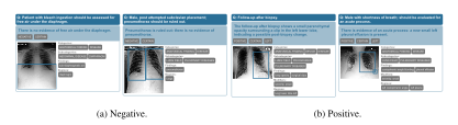
Figure 7: Examples of indication questions. Questions are based on the paraphrased INDICATION section while each main answer is generated based on the indication node from the scene graph.
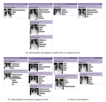
Figure 8: Examples of study abnormality questions. Questions are based on one of 13 templates. Answers may consist of several answer parts, where each describes an individual aspect (about the overall study or a finding category). Individual answer parts are constructed based on observation nodes, filtered based on finding categories relevant to the question, where individual answer parts may be organized hierarchically (indicated by indentations) based on parent-child edges in the scene graph. Additionally assessment answers (b) start with a template-based yes/no answer.
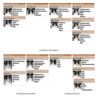
Figure 9: Examples of region abnormality questions. Questions are based on one of 6 templates. Answers may consist of several answer parts, where each describes an individual aspect (about the region). Individual answer parts are constructed based on observation nodes relevant to the region, where individual answer parts may be organized hierarchically (indicated by indentations) based on parent-child edges in the scene graph. Additionally assessment answers (b) start with a template-based yes/no answer. Some templates also ask specifically about devices in the region (c).
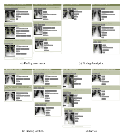
Figure 10: Examples of finding questions. Questions are based on one of 7 templates. Answers start with a template-based answer part to identify the finding presence (a), provide a severity summary (b), describe the location (c), or presence of a device (d). Additional details may be provided in answer parts based on observation nodes relevant to the finding, where individual answer parts may be organized hierarchically (indicated by indentations) based on parent-child edges in the scene graph.
B FURTHER ANALYSIS OF QA-SAMPLES
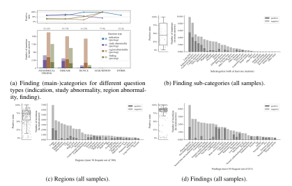
Figure 11: Tags (finding main- and sub-categories, regions, findings) mentioned in answers. We show their positive ratios (top/left), i.e. how often they are mentioned in positive versus in negative answer parts and plot the number of positive and negative mentions of the most frequent tags (bottom/right).
C EVALUATION DETAILS
C.1 QA EVALUATION: ASSESSMENT OF THE LLM- AS- A- JUDGE
| Metric | Entailment | Relevance | Completeness | Question clarity | Answer clarity |
|---|---|---|---|---|---|
| Rating classes | 7 classes | 4 classes | 5 classes | 6 classes | 5 classes |
| % overrated grade | 1% | 0% | 2% | 0% | 0% |
| Cohen’s kappa | 0.49 | 0.65 | 0.41 | 0.32 | 0.32 |
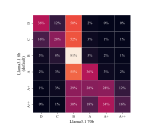
Figure 12: Confusion matrix comparing the assigned quality ratings between using Llama3.1 8b (default) and Llama3.1 70b as an LLM-judge (see Secs. 3.3 and 4.2). In most cases, ratings differ only slightly. Most importantly, low-quality samples (as rated by Llama3.1 70b) are almost never assigned to fine-tuning grades (A or higher) by Llama3.1 8b. We thus decided to use Llama3.1 8b as our default rater, as it is much more computationally efficient.
C.2 SCENE GRAPH EVALUATION: FINDING TAGS
| Chest ImaGenome [MCC] | |||||
|---|---|---|---|---|---|
| Classes | Anat. Find. | Disease | Tubes | Device | Micro |
| Ours (Image-level) | 0.63 | 0.74 | 0.74 | 0.76 | 0.69 |
| Ours (Region-level) | 0.43 | 0.50 | 0.56 | 0.46 | 0.53 |
| Finding | Precision — Ours | Precision — Chest ImaG. | Recall — Ours | Recall — Chest ImaG. | F1 — Ours | F1 — Chest ImaG. | MCC — Ours | MCC — Chest ImaG. |
|---|---|---|---|---|---|---|---|---|
| Findings in CXP-5, CXP-7, and CXP-13 | ||||||||
| Atelectasis | 0.82[0.78, 0.87] | 0.78[0.73, 0.83] | 0.99[0.97, 1.0] | 0.99[0.98, 1.0] | 0.9[0.87, 0.93] | 0.88[0.84, 0.9] | 0.84[0.8, 0.88] | 0.81[0.77, 0.85] |
| Cardiomegaly | 0.64[0.58, 0.7] | 0.67[0.61, 0.74] | 0.85[0.78, 0.9] | 0.82[0.75, 0.87] | 0.73[0.67, 0.78] | 0.74[0.68, 0.79] | 0.61[0.54, 0.68] | 0.63[0.56, 0.69] |
| Consolidation | 0.83[0.73, 0.91] | 0.77[0.68, 0.86] | 0.87[0.79, 0.94] | 0.93[0.86, 0.99] | 0.85[0.78, 0.91] | 0.84[0.78, 0.9] | 0.83[0.75, 0.9] | 0.83[0.76, 0.89] |
| Edema | 0.94[0.9, 0.98] | 0.9[0.85, 0.95] | 0.8[0.73, 0.86] | 0.8[0.74, 0.86] | 0.86[0.82, 0.9] | 0.85[0.8, 0.89] | 0.83[0.77, 0.87] | 0.8[0.74, 0.85] |
| Pleural Effusion | 0.9[0.86, 0.93] | 0.86[0.82, 0.9] | 0.98[0.96, 1.0] | 0.97[0.94, 0.99] | 0.94[0.92, 0.96] | 0.91[0.89, 0.94] | 0.89[0.85, 0.92] | 0.85[0.8, 0.89] |
| Findings in CXP-7 and CXP-13 | ||||||||
| Pneumonia | 0.92[0.87, 0.96] | 0.89[0.84, 0.94] | 0.94[0.89, 0.97] | 0.95[0.91, 0.98] | 0.93[0.89, 0.96] | 0.92[0.89, 0.95] | 0.91[0.87, 0.95] | 0.9[0.86, 0.94] |
| Pneumothorax | 0.78[0.64, 0.89] | 0.79[0.66, 0.91] | 0.84[0.71, 0.95] | 0.89[0.78, 0.98] | 0.8[0.69, 0.89] | 0.84[0.74, 0.92] | 0.79[0.68, 0.88] | 0.83[0.72, 0.91] |
| Findings in CXP-13 | ||||||||
| Enlarged Cardiom. | 0.51[0.37, 0.65] | 0.61[0.41, 0.8] | 0.39[0.29, 0.51] | 0.23[0.13, 0.33] | 0.44[0.34, 0.55] | 0.33[0.2, 0.45] | 0.39[0.28, 0.51] | 0.33[0.19, 0.45] |
| Lung Lesion | 0.17[0.12, 0.22] | 0.68[0.56, 0.79] | 0.81[0.69, 0.91] | 0.87[0.76, 0.95] | 0.28[0.21, 0.35] | 0.76[0.66, 0.84] | 0.25[0.17, 0.32] | 0.74[0.64, 0.83] |
| Lung Opacity | 0.62[0.56, 0.69] | 0.28[0.24, 0.31] | 0.83[0.77, 0.89] | 1.0[1.0, 1.0] | 0.71[0.65, 0.76] | 0.43[0.39, 0.48] | 0.61[0.54, 0.68] | 0.2[0.17, 0.23] |
| Pleural Other | 0.54[0.36, 0.71] | 0.3[0.19, 0.42] | 0.87[0.7, 1.0] | 0.92[0.76, 1.0] | 0.67[0.49, 0.8] | 0.45[0.31, 0.58] | 0.67[0.51, 0.79] | 0.5[0.37, 0.6] |
| Fracture | 0.67[0.54, 0.79] | 0.6[0.47, 0.73] | 0.92[0.82, 1.0] | 0.82[0.68, 0.93] | 0.77[0.67, 0.86] | 0.69[0.58, 0.79] | 0.77[0.67, 0.85] | 0.68[0.56, 0.78] |
| Support Devices | 0.61[0.56, 0.66] | 0.62[0.56, 0.67] | 0.98[0.96, 1.0] | 0.83[0.77, 0.88] | 0.75[0.71, 0.79] | 0.71[0.66, 0.75] | 0.63[0.59, 0.68] | 0.54[0.48, 0.61] |
| Macro-averages | ||||||||
| CheXpert-5 (CXP-5) | 0.83[0.79, 0.85] | 0.8[0.77, 0.83] | 0.9[0.87, 0.92] | 0.9[0.88, 0.92] | 0.85[0.83, 0.87] | 0.84[0.82, 0.86] | 0.8[0.77, 0.82] | 0.78[0.75, 0.81] |
| CheXpert-7 (CXP-7) | 0.83[0.8, 0.86] | 0.81[0.78, 0.84] | 0.89[0.87, 0.92] | 0.91[0.88, 0.93] | 0.86[0.83, 0.88] | 0.85[0.83, 0.87] | 0.81[0.79, 0.84] | 0.8[0.78, 0.83] |
| CheXpert-13 (CXP-13) | 0.69[0.66, 0.71] | 0.67[0.65, 0.7] | 0.85[0.83, 0.87] | 0.85[0.82, 0.87] | 0.74[0.72, 0.76] | 0.72[0.7, 0.74] | 0.69[0.67, 0.71] | 0.66[0.64, 0.69] |
| Micro | 0.68[0.66, 0.7] | 0.63[0.61, 0.65] | 0.89[0.87, 0.9] | 0.88[0.86, 0.89] | 0.77[0.75, 0.79] | 0.73[0.72, 0.75] | 0.71[0.69, 0.73] | 0.67[0.65, 0.68] |
| Finding | Precision — Ours | Precision — Chest ImaG. | Recall — Ours | Recall — Chest ImaG. | F1 — Ours | F1 — Chest ImaG. | MCC — Ours | MCC — Chest ImaG. |
|---|---|---|---|---|---|---|---|---|
| Findings in CXP-5, CXP-7, CXP-13, and CXR-LT | ||||||||
| Atelectasis | 0.55[0.47, 0.62] | 0.56[0.49, 0.61] | 0.82[0.75, 0.88] | 0.99[0.97, 1.0] | 0.66[0.59, 0.71] | 0.71[0.65, 0.76] | 0.48[0.4, 0.57] | 0.59[0.54, 0.65] |
| Cardiomegaly | 0.82[0.76, 0.88] | 0.85[0.79, 0.91] | 0.85[0.79, 0.91] | 0.8[0.73, 0.86] | 0.84[0.79, 0.88] | 0.82[0.77, 0.87] | 0.73[0.66, 0.79] | 0.72[0.65, 0.79] |
| Consolidation | 0.82[0.73, 0.91] | 0.74[0.63, 0.83] | 0.86[0.76, 0.93] | 0.89[0.8, 0.95] | 0.84[0.77, 0.9] | 0.8[0.73, 0.87] | 0.8[0.72, 0.87] | 0.76[0.67, 0.83] |
| Edema | 0.73[0.63, 0.83] | 0.69[0.6, 0.79] | 0.64[0.55, 0.74] | 0.71[0.61, 0.8] | 0.68[0.6, 0.76] | 0.7[0.62, 0.77] | 0.59[0.5, 0.69] | 0.6[0.5, 0.69] |
| Pleural Effusion | 0.82[0.76, 0.87] | 0.78[0.73, 0.84] | 0.93[0.9, 0.97] | 0.97[0.94, 0.99] | 0.87[0.83, 0.91] | 0.87[0.83, 0.9] | 0.77[0.7, 0.82] | 0.76[0.7, 0.82] |
| Findings in CXP-7, CXP-13, and CXR-LT | ||||||||
| Pneumonia | 0.38[0.19, 0.58] | 0.13[0.07, 0.21] | 0.45[0.25, 0.67] | 0.76[0.55, 0.94] | 0.41[0.22, 0.58] | 0.23[0.13, 0.33] | 0.38[0.19, 0.55] | 0.24[0.13, 0.34] |
| Pneumothorax | 0.85[0.73, 0.95] | 0.8[0.7, 0.9] | 0.85[0.72, 0.94] | 0.96[0.89, 1.0] | 0.85[0.75, 0.92] | 0.87[0.8, 0.94] | 0.83[0.72, 0.91] | 0.86[0.78, 0.93] |
| Findings in CXP-13 and CXR-LT | ||||||||
| Enlarged Cardiom. | 0.78[0.57, 0.95] | 1.0[1.0, 1.0] | 0.13[0.07, 0.2] | 0.1[0.05, 0.17] | 0.22[0.13, 0.32] | 0.18[0.1, 0.29] | 0.24[0.13, 0.35] | 0.27[0.19, 0.36] |
| Lung Lesion | 0.01[0.0, 0.03] | 0.05[0.0, 0.12] | 0.5[0.0, 1.0] | 0.75[0.0, 1.0] | 0.02[0.0, 0.06] | 0.1[0.0, 0.22] | 0.0[-0.09, 0.1] | 0.18[-0.02, 0.3] |
| Lung Opacity | 0.92[0.87, 0.96] | 0.54[0.49, 0.59] | 0.77[0.72, 0.84] | 1.0[1.0, 1.0] | 0.84[0.8, 0.88] | 0.7[0.66, 0.74] | 0.73[0.66, 0.79] | 0.35[0.29, 0.4] |
| Pleural Other | 0.11[0.0, 0.24] | 0.23[0.13, 0.34] | 0.19[0.0, 0.43] | 1.0[1.0, 1.0] | 0.14[0.0, 0.29] | 0.38[0.23, 0.51] | 0.1[-0.05, 0.26] | 0.45[0.34, 0.55] |
| Fracture | 0.89[0.78, 0.98] | 0.84[0.72, 0.94] | 0.91[0.81, 0.98] | 0.82[0.69, 0.93] | 0.9[0.82, 0.95] | 0.83[0.73, 0.9] | 0.89[0.8, 0.95] | 0.81[0.69, 0.89] |
| Support Devices | 0.92[0.88, 0.96] | 0.93[0.9, 0.97] | 0.93[0.89, 0.96] | 0.83[0.77, 0.88] | 0.92[0.9, 0.95] | 0.88[0.84, 0.91] | 0.83[0.77, 0.88] | 0.75[0.68, 0.82] |
| Findings in LT-only, and CXR-LT | ||||||||
| Calcification of Aorta | 0.95[0.83, 1.0] | 0.95[0.88, 1.0] | 0.43[0.28, 0.58] | 0.93[0.85, 1.0] | 0.6[0.43, 0.73] | 0.94[0.89, 0.99] | 0.61[0.48, 0.73] | 0.94[0.87, 0.99] |
| Emphysema | 0.58[0.41, 0.74] | 0.54[0.38, 0.69] | 0.81[0.63, 0.95] | 0.81[0.63, 0.95] | 0.68[0.52, 0.8] | 0.65[0.49, 0.77] | 0.66[0.5, 0.79] | 0.63[0.47, 0.75] |
| Fibrosis | 0.27[0.15, 0.43] | 0.0[0.0, 0.0] | 0.52[0.31, 0.74] | 0.0[0.0, 0.0] | 0.36[0.21, 0.52] | 0.0[0.0, 0.0] | 0.33[0.17, 0.5] | 0.0[0.0, 0.0] |
| Hernia | 1.0[1.0, 1.0] | 0.86[0.68, 1.0] | 0.9[0.73, 1.0] | 0.9[0.73, 1.0] | 0.95[0.85, 1.0] | 0.88[0.74, 0.97] | 0.95[0.85, 1.0] | 0.87[0.73, 0.97] |
| Infiltration | 0.15[0.03, 0.3] | 0.38[0.16, 0.67] | 0.33[0.08, 0.7] | 0.55[0.21, 0.88] | 0.21[0.05, 0.39] | 0.44[0.18, 0.69] | 0.19[0.01, 0.39] | 0.44[0.17, 0.69] |
| Mass | 0.54[0.34, 0.74] | 0.28[0.17, 0.4] | 0.78[0.56, 0.94] | 0.89[0.71, 1.0] | 0.64[0.44, 0.78] | 0.42[0.28, 0.56] | 0.63[0.45, 0.77] | 0.46[0.32, 0.58] |
| Nodule | 0.92[0.79, 1.0] | 0.5[0.36, 0.63] | 0.74[0.57, 0.88] | 0.91[0.78, 1.0] | 0.82[0.68, 0.91] | 0.64[0.51, 0.75] | 0.81[0.68, 0.91] | 0.64[0.51, 0.74] |
| Pleural Thickening | 0.78[0.62, 0.92] | 0.33[0.22, 0.45] | 1.0[1.0, 1.0] | 1.0[1.0, 1.0] | 0.88[0.77, 0.96] | 0.5[0.36, 0.62] | 0.88[0.78, 0.96] | 0.54[0.43, 0.64] |
| Pneumomediastinum | 0.94[0.83, 1.0] | 0.88[0.73, 0.97] | 0.84[0.7, 0.96] | 0.84[0.7, 0.96] | 0.89[0.78, 0.96] | 0.86[0.73, 0.94] | 0.88[0.77, 0.95] | 0.85[0.72, 0.93] |
| Pneumoperitoneum | 0.88[0.72, 1.0] | 0.82[0.65, 0.96] | 0.96[0.85, 1.0] | 1.0[1.0, 1.0] | 0.92[0.81, 1.0] | 0.9[0.79, 0.98] | 0.91[0.8, 1.0] | 0.9[0.8, 0.98] |
| Subcut. Emphysema | 0.97[0.9, 1.0] | 0.0[0.0, 0.0] | 0.8[0.68, 0.92] | 0.0[0.0, 0.0] | 0.88[0.79, 0.95] | 0.0[0.0, 0.0] | 0.87[0.78, 0.94] | 0.0[0.0, 0.0] |
| Tortuous Aorta | 0.83[0.69, 0.95] | 0.79[0.64, 0.91] | 0.88[0.75, 0.97] | 0.94[0.84, 1.0] | 0.85[0.75, 0.93] | 0.86[0.75, 0.94] | 0.84[0.73, 0.93] | 0.85[0.74, 0.93] |
| Macro-averages | ||||||||
| CheXpert-5 (CXP-5) | 0.75[0.71, 0.78] | 0.72[0.69, 0.76] | 0.82[0.79, 0.85] | 0.87[0.84, 0.9] | 0.78[0.75, 0.8] | 0.78[0.75, 0.81] | 0.67[0.64, 0.71] | 0.69[0.65, 0.72] |
| CheXpert-7 (CXP-7) | 0.71[0.66, 0.75] | 0.65[0.62, 0.68] | 0.77[0.73, 0.81] | 0.87[0.83, 0.9] | 0.73[0.7, 0.77] | 0.71[0.69, 0.74] | 0.65[0.61, 0.69] | 0.65[0.61, 0.68] |
| CheXpert-13 (CXP-13) | 0.66[0.63, 0.69] | 0.63[0.61, 0.65] | 0.68[0.63, 0.73] | 0.81[0.75, 0.85] | 0.63[0.6, 0.65] | 0.62[0.6, 0.64] | 0.57[0.54, 0.6] | 0.56[0.54, 0.59] |
| LT-only | 0.73[0.69, 0.77] | 0.53[0.48, 0.57] | 0.75[0.7, 0.8] | 0.73[0.69, 0.77] | 0.72[0.68, 0.75] | 0.59[0.55, 0.62] | 0.71[0.67, 0.74] | 0.59[0.55, 0.63] |
| CXR-LT | 0.7[0.67, 0.72] | 0.58[0.56, 0.6] | 0.71[0.68, 0.75] | 0.77[0.74, 0.8] | 0.67[0.65, 0.69] | 0.61[0.58, 0.62] | 0.64[0.61, 0.66] | 0.58[0.55, 0.6] |
| Micro | 0.69[0.67, 0.71] | 0.62[0.6, 0.64] | 0.76[0.74, 0.78] | 0.8[0.78, 0.82] | 0.72[0.71, 0.74] | 0.7[0.68, 0.72] | 0.67[0.65, 0.69] | 0.64[0.62, 0.66] |
C.3 SCENE GRAPH EVALUATION: FINDING BOXES
| Finding | IoU@30 — Ours | IoU@30 — Chest ImaG. | IoP@30 — Ours | IoP@30 — Chest ImaG. | IoT@30 — Ours | IoT@30 — Chest ImaG. |
|---|---|---|---|---|---|---|
| Atelectasis | 0.28[0.12, 0.42] | 0.1[0.02, 0.2] | 0.5[0.34, 0.66] | 0.14[0.05, 0.28] | 0.83[0.71, 0.93] | 0.85[0.74, 0.94] |
| Cardiomegaly | 0.96[0.93, 0.98] | 0.97[0.95, 0.99] | 1.0[1.0, 1.0] | 1.0[1.0, 1.0] | 0.96[0.93, 0.98] | 0.99[0.98, 1.0] |
| Consolidation | 0.31[0.19, 0.45] | 0.2[0.1, 0.31] | 0.41[0.29, 0.54] | 0.24[0.12, 0.35] | 0.91[0.81, 0.98] | 0.98[0.93, 1.0] |
| Edema | 0.52[0.32, 0.71] | 0.52[0.32, 0.71] | 0.52[0.32, 0.71] | 0.52[0.32, 0.71] | 1.0[1.0, 1.0] | 1.0[1.0, 1.0] |
| Pneumonia | 0.48[0.41, 0.57] | 0.28[0.21, 0.35] | 0.58[0.5, 0.66] | 0.34[0.26, 0.42] | 0.93[0.88, 0.97] | 1.0[1.0, 1.0] |
| Pneumothorax | 0.14[0.1, 0.18] | 0.15[0.1, 0.2] | 0.14[0.1, 0.19] | 0.15[0.11, 0.2] | 0.96[0.93, 0.98] | 0.98[0.96, 1.0] |
| Macro | 0.45[0.4, 0.5] | 0.37[0.33, 0.41] | 0.53[0.48, 0.58] | 0.4[0.36, 0.44] | 0.93[0.9, 0.95] | 0.97[0.95, 0.98] |
| Micro | 0.51[0.47, 0.54] | 0.45[0.42, 0.49] | 0.56[0.52, 0.6] | 0.48[0.45, 0.52] | 0.94[0.92, 0.96] | 0.98[0.97, 0.99] |
| Finding | IoU@30 — Ours | IoU@30 — Chest ImaG. | IoP@30 — Ours | IoP@30 — Chest ImaG. | IoT@30 — Ours | IoT@30 — Chest ImaG. |
|---|---|---|---|---|---|---|
| Abnormal mediastinal contour | 0.08[0.0, 0.31] | 0.25[0.0, 0.57] | 0.08[0.0, 0.31] | 0.25[0.0, 0.57] | 1.0[1.0, 1.0] | 1.0[1.0, 1.0] |
| Acute fracture | 0.0[0.0, 0.0] | 0.0[0.0, 0.0] | 0.0[0.0, 0.0] | 0.0[0.0, 0.0] | 1.0[1.0, 1.0] | 0.0[0.0, 0.0] |
| Atelectasis | 0.29[0.26, 0.33] | 0.15[0.12, 0.17] | 0.47[0.44, 0.51] | 0.2[0.17, 0.23] | 0.76[0.73, 0.78] | 0.93[0.91, 0.94] |
| Consolidation | 0.39[0.33, 0.45] | 0.27[0.22, 0.32] | 0.51[0.45, 0.57] | 0.34[0.28, 0.4] | 0.8[0.74, 0.85] | 0.95[0.92, 0.97] |
| Emphysema | 1.0[1.0, 1.0] | 1.0[1.0, 1.0] | 1.0[1.0, 1.0] | 1.0[1.0, 1.0] | 1.0[1.0, 1.0] | 1.0[1.0, 1.0] |
| Enlarged cardiac silhouette | 0.96[0.94, 0.97] | 0.96[0.95, 0.97] | 1.0[0.99, 1.0] | 0.99[0.99, 1.0] | 0.96[0.95, 0.97] | 0.98[0.97, 0.99] |
| Enlarged hilum | 0.5[0.0, 1.0] | 0.5[0.0, 1.0] | 0.5[0.0, 1.0] | 0.8[0.23, 1.0] | 0.5[0.0, 1.0] | 0.5[0.0, 1.0] |
| Fracture | 0.0[0.0, 0.0] | 0.0[0.0, 0.0] | 0.0[0.0, 0.0] | 0.0[0.0, 0.0] | 0.0[0.0, 0.0] | 0.0[0.0, 0.0] |
| Groundglass opacity | 0.28[0.22, 0.34] | 0.31[0.25, 0.38] | 0.48[0.4, 0.54] | 0.38[0.32, 0.45] | 0.77[0.71, 0.83] | 0.96[0.93, 0.99] |
| Hiatal hernia | 0.19[0.0, 0.43] | 0.4[0.17, 0.67] | 0.27[0.06, 0.5] | 0.4[0.17, 0.67] | 0.94[0.78, 1.0] | 1.0[1.0, 1.0] |
| High lung volume / emphysema | 0.48[0.25, 0.7] | 0.58[0.35, 0.79] | 0.58[0.35, 0.79] | 0.58[0.35, 0.79] | 0.9[0.75, 1.0] | 1.0[1.0, 1.0] |
| Interstitial lung disease | 0.5[0.0, 1.0] | 0.8[0.0, 1.0] | 0.8[0.0, 1.0] | 0.8[0.0, 1.0] | 0.8[0.12, 1.0] | 1.0[1.0, 1.0] |
| Lung nodule or mass | 0.18[0.08, 0.31] | 0.09[0.02, 0.2] | 0.21[0.1, 0.35] | 0.09[0.02, 0.2] | 0.89[0.77, 0.97] | 0.91[0.8, 0.98] |
| Pleural abnormality | 0.16[0.13, 0.19] | 0.14[0.11, 0.17] | 0.2[0.17, 0.23] | 0.17[0.14, 0.2] | 0.91[0.88, 0.93] | 0.92[0.9, 0.94] |
| Pleural effusion | 0.42[0.2, 0.65] | 0.37[0.17, 0.6] | 0.53[0.3, 0.75] | 0.53[0.31, 0.75] | 1.0[1.0, 1.0] | 0.95[0.82, 1.0] |
| Pleural thickening | 0.0[0.0, 0.0] | 0.0[0.0, 0.0] | 0.0[0.0, 0.0] | 0.0[0.0, 0.0] | 1.0[1.0, 1.0] | 1.0[1.0, 1.0] |
| Pneumothorax | 0.04[0.01, 0.08] | 0.13[0.07, 0.21] | 0.04[0.01, 0.08] | 0.13[0.07, 0.21] | 0.9[0.84, 0.96] | 0.96[0.92, 0.99] |
| Pulmonary edema | 0.51[0.45, 0.56] | 0.58[0.53, 0.63] | 0.55[0.5, 0.6] | 0.58[0.53, 0.63] | 0.95[0.93, 0.97] | 1.0[1.0, 1.0] |
| Macro | 0.34[0.27, 0.42] | 0.37[0.3, 0.45] | 0.41[0.34, 0.49] | 0.41[0.33, 0.49] | 0.84[0.78, 0.91] | 0.87[0.8, 0.95] |
| Micro | 0.45[0.44, 0.47] | 0.42[0.4, 0.43] | 0.54[0.53, 0.56] | 0.46[0.44, 0.47] | 0.87[0.86, 0.88] | 0.95[0.94, 0.96] |
D DATASET STRUCTURE
D.1 SCENE GRAPH STRUCTURE
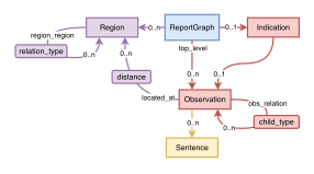
Figure 13: Scene graph structure overview.
Sentence Nodes Sentence nodes are directly associated with raw sentences in the report, i.e. there is exactly one sentence node per identified report sentence. They contain the following attributes:
- sent id: Identifier, unique per study. Example: S01. • section: Name of the section that the sentence belongs to, as specified in the report. If the sentence is not part of a section, FINAL REPORT NO SECTION or PRE FINAL REPORT NO SECTION are used. Examples: FINDINGS, IMPRESSION, REASON FOR EXAM. • section type: The identified type of section used for classifying the type of content of the sentence. IGNORE is used for irrelevant sections. Examples: FINDINGS, IMPRESSION, INDICATION. • sentence: The raw sentence as written in the report.
Observation Nodes Observation nodes are created for each individually described aspect (i.e. observation) in the report’s FINDINGS or IMPRESSION section. Hereby, a single sentence may be related to several observation nodes and a single observation may be derived from several sentences (if they describe related aspects). Observation nodes are structured hierarchically, i.e. they may have other observation nodes as parents. An observation node contains the following attributes:
- obs id: Identifier, unique per study. Example: O01. For child nodes this also contains the parent id, e.g. O01.02. • summary sentence: Textual description of the observation, directly derived from the associated report sentences. In some cases, this may be an exact copy of the report sentences but it may also paraphrase parts of it. • name: Abbreviated version of the summary sentence. • child level: Hierarchy level, 0 for top-level, larger numbers for deeper hierarchy levels. • child type: Type of parent-child relation. Possible options: regional distinction, related region, associated with, device part, recommendation, comparison only. • regions: List of associated regions, each paired with an optional list of distance annotations. Example: [("heart", ["1 cm above"])] • non resolved regions: Similar to regions but with regions that could not be semantically mapped to reference definitions.
laterality: Laterality of the region. Possible options:left,right,likely bilateral,bilateral,unknown.default_regions: List of regions that have been added because they are defaults for the identified findings (obs_entities).obs_entities: List of (directly) associated findings. Example:["pleural effusion"].obs_entities_parents: List of findings that are considered parents of findings inobs_entities.non_resolved_obs_entities: Similar toobs_entitiesbut with findings that could not be semantically mapped to reference definitions.obs_categories: List of associated finding super-categories. Example:["ANATOMICAL_FINDING"].obs_subcategories: List of associated finding sub-categories. Example:["LUNG_FIELD"].probability: Likelihood of the observation being positive. Short term, derived from what is mentioned in the report.certainty: How certain is the observation. Derived fromprobability. Possible options:certain,likely,uncertain,comparison_only,recommendation.positiveness: Whether the observation is positive or negative. Derived fromprobability. Possible options:pos,neg,comparison_only,recommendation.modifiers: Modifiers of the finding. Dictionary with keys for each type of modifier and lists of the individual modifier values. Possible modifier type:severity,texture,spread,temporal. Example:{"severity": ["mild"], "spread": ["focal"]}.change_sentence: Optional textual description of any changes to the prior study of the same patient, if it was mentioned in the report.changes: List of change types mentioned in thechange_sentence. Example:worsening.from_report: Whether this observation was explicitly mentioned in the report (true) or automatically added (false).obs_quality: Extraction quality of the observation, consisting of several individual aspects. See Tab. 11.localization: Bounding boxes for this observation, for each associated image. Dictionary with keys equaling image ids (each study may correspond to several images). Values contain:image_idbboxes: List of bounding boxes in the(x1, y1, x2, y2)format in original image-pixel coordinates.localization_reference_ids: List of region names from which the bounding boxes are derived.missing_localization: List of associated region names for which no localization is available for this image.is_fallback: Whether this localization is a fallback, i.e. the original region localization was not available but a more coarse localization was used instead.localization_quality: Quality of the localization. See Tab. 11.
Region Nodes Region nodes are created for each anatomical structure mentioned in any observation and for key regions. They contain the following attributes:
- region: Name of the region and unique identifier within each study. Example: left lung.
- laterality: Laterality of the region. Possible options: left, right, bilateral, unknown (i.e. not clearly definable).
- localization: Bounding boxes for this region, for each associated image. Same format as for observation nodes.
- region localization quality: Quality of the localization attribute. See Tab. 11.
Indication Node Each study contains an optional indication node with information extracted from the INDICATION section. If present, it contains the following attributes:
- indication summary: Summary of the indication, directly derived from the INDICATION section of the report, but typically paraphrased.
- patient info: Any information about the patient, if mentioned in the INDICATION section. A subset of the content in indication summary.
- indication: Indication for the study, if mentioned in the INDICATION section. A subset of the content in indication summary.
- evaluation: Any required evaluation of the patient (i.e. what should be evaluated with this study), if mentioned in the INDICATION section. A subset of the content in indication summary.
- associated sentence ids: List of sent ids from sentence nodes that are related to the indication.
- associated obs ids: List of obs ids from observation nodes that are related to the indication.
- answer for indication: A single observation node containing the answer to the question (implicitly) asked by the provided indication. This is a special observation node with obs id = OIND. Its textual description is directly derived from the FINDINGS and IMPRESSION sections but conditioned on the INDICATION section.
Root Node and Relations Each study contains a single root node called the ReportGraph. It contains general metadata about the study and its scene graphs:
- patient id: Unique patient ID, the subject id from MIMIC-CXR.
- study id: Unique study ID, from MIMIC-CXR. Each patient may have several studies.
- study quality: The overall extraction quality of the scene graph for this study, consisting of several individual aspects. See Tab. 11.
- study img localization quality: Dictionary of localization qualities for each image with keys corresponding to image IDs. See Tab. 11.
Additionally, it is connected to all other nodes and links to the top-level (root) observations. Thus, it contains the following:
- sentences: List of all sentence nodes.
- observations: Dictionary of all observation nodes, indexed by their obs id.
- top level obs ids: List of all top-level (root) observation node IDs, i.e. their obs ids.
- regions: Dictionary of all region nodes, indexed by their region attribute.
- indication: The indication node, if it exists.
Nodes can also be connected by the following relations:
- located at relations (observation↔region): Specifies where an observation is located with the following additional attributes:
– distances: List of distance annotations, e.g. ["3cm above"]. – where specified: How this relation was derived. Possible options: direct, bilateral, sub region.
- obs relations (observation↔observation): Specifies a parent-child relation between two observations, with the following additional attribute:
– child type: Type of parent-child relation. Possible options: regional distinction, related region, associated with, device part, recommendation, comparison only.
- obs sent relations (observation↔sentence): Specifies from which sentences an observation was derived.
- region region relations (region↔region): Specifies a relation between two regions with the following additional attribute:
– relation type: Type of relation. Possible options: sub region, bilateral (the bilateral version of a region), left (the left version of a region), right (the right version of a region).
D.2 QUESTION-ANSWER STRUCTURE
QA-Pair Each question-answer pair consists of a free-text question (attribute question), an answer consisting of structured answer parts (attribute answers). Additionally, it contains the following metadata:
- question id: Identifier, unique within the associated study.
- question type: The QA-template used to generate this QA-pair.
- question strategy: The strategy used to generate QA-pair. See Secs. 3.2 and E.2.2.
- variables: Key-value pairs of variables (and their values) used during generation, e.g. to fill the template. See Sec. E.2.1.
- obs ids: List of obs idss of observation nodes (in the scene graph) from which the answer is derived.
- contains report answers: Whether any of the answer parts was derived from the report, i.e. from observation nodes.
- contains template answers: Whether any of the answer parts was generated based on a template.
- extraction quality: The overall extraction quality of the associated observations in the scene graph, consisting of several individual aspects. See Tab. 11.
- question img localization quality: Quality of the localizations per image. See Tab. 11.
- question quality: The overall question-answer text quality, consisting of several individual aspects. See Tab. 12.
- rating: The overall rating of the QA-pair. See Sec. D.3
Answers are structured hierarchically, consisting of a list of answer parts (attribute answers) and sub-answers (children) of these answers, where there can be several hierarchy levels. The hierarchy levels are derived from the parent-child structure of associated observation nodes (based on obs relations, Sec. D.1). Additionally, there are different types of answer parts:
- main answer: Required to answer the question. There is always at least one main-answer per question.
- details: Providing additional details for the main answer, which are however not mandatory to answer the question.
- related information: Not directly answering the question, but may be related and provides context.
Each individual answer part contains the following attributes:
- answer id: Identifier, unique within each study. Contains the question id.
text: The answer text. Either generated from a template or based onsummary_sentencein the observation node (Sec. D.1).answer_level: Hierarchy level, 0 for top-level answer part, larger numbers for deeper hierarchy levels (sub-answers).answer_type: Type of answer part. Possible options:main_answer,details,related_information.name_tag: Abbreviated version of thetext. Either generated from a template or based onnamein the observation node (Sec. D.1).laterality: Laterality of the region. See observation node (Sec. D.1). Possible options:left,right,likely bilateral,bilateral,unknown.regions: List of associated regions. See observation node (Sec. D.1). Distances are not provided here. Example:["heart"].obs_entities: List of (directly) associated findings. See observation node (Sec. D.1). Example:["pleural effusion"].obs_entities_parents: List of findings that are considered parents of findings inobs_entities. See observation node (Sec. D.1).obs_categories: List of associated finding super-categories. See observation node (Sec. D.1). Example:["ANATOMICAL_FINDING"].obs_subcategories: List of associated finding sub-categories. See observation node (Sec. D.1). Example:["LUNG_FIELD"].certainty: How certain is the observation. See observation node (Sec. D.1). Possible options:certain,likely,uncertain,comparison_only,recommendation.positiveness: Whether the observation is positive or negative. See observation node (Sec. D.1). Possible options:pos,neg,comparison_only,recommendation.modifiers: Modifiers of the finding. List of pairs of modifier type and value. See observation node (Sec. D.1). Possible modifier type:severity,texture,spread,temporal. Example:[("severity", "mild"), ("spread", "focal")].localization: Bounding boxes for this answer part, for each associated image. Dictionary with keys equaling image ids (each study may correspond to several images). See observation node (Sec. D.1).sub_answers: List of child answers (deeper in the hierarchy). Each sub-answer is another answer-part with all attributes and potentially further sub-answers.from_report: Whether this answer part is derived from the report, i.e. an observation node (true), or from a template (false).extraction_quality: The overall extraction quality of the associated observations in the scene graph, consisting of several individual aspects. See Tab. 11.answer_quality: The overall answer text quality, consisting of several individual aspects. See Tab. 12.
D.3 QUALITY
Ratings
We distinguish between the following overall ratings for each QA-pair:
- A++: Perfect and complete content; all information in the answer is explicitly mentioned in the report. • A+: Perfect and mostly complete content; all information in the answer is explicitly mentioned in the report, but some minor details may be missing or irrelevant.
- A: Very good content with minor issues not affecting the overall quality; some tags or boxes may be inferred or minor issues (e.g. grammatical) may be present in the text.
- B: Good content; factually correct answers, which may however be not fully complete or slightly unclear.
- C: Poor content; answers may be misleading or contain completely unclear information.
- D: Incorrect content; answers may be contradicting the report and are not usable.
- not rated: Quality could not be assessed, e.g. due to invalid LLM-rater outputs.
These ratings are derived based on individual aspects that will be described in the following paragraphs. Possible quality levels for each aspects and the resulting rating are presented in Tabs. 11 and 12. The final rating is computed as the minimum (worst) rating over all individual aspects.
Scene Graph Extraction Quality For each scene graph, we provide a quality rating based on how well it could be constructed/extracted. Tab. 11 shows the considered aspects with their potential quality levels and resulting ratings.
| Aspect | Quality level | Value | Resulting rating |
|---|---|---|---|
| Region extraction — How well are region tags identified? (attribute regions) | |||
| Region extraction | NO REGIONS | 0 | B |
| Region extraction | DEFAULT REGIONS ONLY | 1 | B |
| Region extraction | CONTAINS DEFAULT REGIONS | 2 | A |
| Region extraction | CONTAINS NON RESOLVED REGIONS | 3 | A |
| Region extraction | RESOLVED REGIONS ONLY | 4 | A++ |
| Finding extraction — How well are finding tags identified? (attribute obs entities) | |||
| Finding extraction | NO ENTITIES | 0 | B |
| Finding extraction | CONTAINS NON RESOLVED ENTITIES | 1 | A |
| Finding extraction | RESOLVED ENTITIES ONLY | 2 | A++ |
| Description extraction — How well are textual descriptions extracted? (attributes summary sentence and name) | |||
| Description extraction | CHANGE IN SENTENCE OR NAME | 0 | B |
| Description extraction | UNDERSCORES IN SENTENCE OR NAME | 1 | A |
| Description extraction | NO ISSUES | 2 | A++ |
| Change extraction — How well are mentions of change extracted? (attributes change sentence and change) | |||
| Change extraction | CHANGE SENTENCE REMOVED | 0 | B |
| Change extraction | UNDERSCORES IN CHANGE SENTENCE | 1 | A |
| Change extraction | CONTAINS NON RESOLVED CHANGES | 2 | A |
| Change extraction | NO ISSUES | 3 | A++ |
| Extraction issues — Have there been any issues in the extraction and scene graph construction pipeline? | |||
| Extraction issues | DISCARDED | -1 | D |
| Extraction issues | NON INTERPRETABLE | 0 | C |
| Extraction issues | MOSTLY INTERPRETABLE | 1 | B |
| Extraction issues | IGNORABLE | 2 | A |
| Extraction issues | FIXABLE | 3 | A+ |
| Extraction issues | NO ISSUES | 4 | A++ |
| Localization — How well could observations/regions be localized? (attribute localization) | |||
| Localization | NO LOCALIZATION | 0 | B |
| Localization | FALLBACK LOCALIZATION | 1 | B |
| Localization | INCOMPLETE LOCALIZATION | 2 | A |
| Localization | BBOX LOCALIZATION | 3 | A++ |
| Localization | BBOX AND MASK LOCALIZATION | 4 | A++ |
QA Text Quality For each QA-pair, we provide quality rating for its text, i.e. the question text and the textual descriptions in its answer parts. Tab. 12 shows the considered aspects with their potential quality levels and resulting ratings.
| Aspect | Quality level | Value | Resulting rating |
|---|---|---|---|
| Entailment — Does the answer factually align with the original report? (rated per answer-part, given the question and the report) | |||
| Entailment | NON ALIGNED CONTRADICTING | -3 | D |
| Entailment | NON ALIGNED MISLEADING | -2 | C |
| Entailment | NON ALIGNED NON INFERABLE | -1 | B |
| Entailment | ALIGNED GENERAL STATEMENT | 0 | A |
| Entailment | ALIGNED NEGATIVE NOT MENTIONED | 1 | A+ |
| Entailment | ALIGNED INFERABLE | 2 | A++ |
| Entailment | ALIGNED MENTIONED | 3 | A++ |
| Relevance — Is the answer relevant for the given question? (rated per answer-part, given the question but independent of the report) | |||
| Relevance | IRRELEVANT INFO | -2 | A |
| Relevance | REDUNDANT INFO | -1 | A |
| Relevance | RELATED INFO | 0 | A+ (A++ for related information answer) |
| Relevance | RELEVANT MAIN ANSWER | 1 | A++ (A for related information answer) |
| Completeness — Does the answer cover all aspects in the report that are relevant to the question? (rated for the full answer, given the question and the report) | |||
| Completeness | INCOMPLETE MISLEADING | -2 | C |
| Completeness | INCOMPLETE NON MISLEADING | -1 | B |
| Completeness | NOT ANSWERED | 0 | B |
| Completeness | DETAILS MISSING | 1 | A+ |
| Completeness | FULLY COMPLETE | 2 | A++ |
| Question clarity — Is the generated question clear and grammatically correct? (rated for the question, given nothing else) | |||
| Question clarity | UNANSWERABLE | -3 | C |
| Question clarity | UNRELATED TO CHEST XRAY | -2 | B |
| Question clarity | UNCLEAR QUESTION | -1 | B |
| Question clarity | GRAMMATICAL ERRORS | 0 | A |
| Question clarity | UNUSUAL SENTENCE STRUCTURE | 1 | A |
| Question clarity | OPTIMAL | 2 | A++ |
| Answer clarity — Is the answer clear and grammatically correct? (rated per answer-part, given nothing else) | |||
| Answer clarity | NOT UNDERSTANDABLE | -2 | C |
| Answer clarity | UNCLEAR ANSWER | -1 | B |
| Answer clarity | GRAMMATICAL ERRORS | 0 | A |
| Answer clarity | UNUSUAL SENTENCE STRUCTURE | 1 | A |
| Answer clarity | OPTIMAL | 2 | A++ |
E DATASET CONSTRUCTION DETAILS
E.1 SCENE GRAPH CONSTRUCTION
E.1.1 REGION LOCALIZATION
We use the CXAS (Seibold et al., 2022; 2023) model to predict segmentation masks of 158 anatomical structures on the 377,110 CXRs from MIMIC-CXR-JPG (Johnson et al., 2024a; 2019b; Goldberger et al., 2000). Additionally, we use the bounding boxes provided by the Chest ImaGenome (Wu et al., 2021a;b; Goldberger et al., 2000) dataset, which are provided for 29 anatomical structures in most frontal images of MIMIC-CXR. The masks predicted by CXAS are post-processed with morphological operations to filter out outlier pixels.
We specify 257 localized regions in our reference definitions. For each of these regions, we define how the bounding boxes are derived. We consider the following options:
- CXAS masks: Some regions are directly associated with one of the 158 anatomical structures for which the CXAS model predicts segmentation masks. In these cases, we compute the bounding box around the predicted segmentation mask.
- Chest ImaGenome boxes: Some regions are directly associated with one of the 29 anatomical structures for which Chest ImaGenome provides bounding boxes. In such cases, we use these provided bounding boxes if no CXAS masks are associated.
- Bilateral regions: Some regions refer to a pair of bilateral regions (e.g. lungs refers to left lung and right lung). In these cases, we simply use the two bounding boxes of the left and right versions, but do not fuse them.
- Parent regions: For some regions we do not have exact correspondences to available masks or boxes but we have available sub-regions. In these cases, we compute the super bounding box, a single box, around all specified child regions.
- Fusions: In some rare cases, we combine multiple individual masks or bounding boxes. We compute intersections or unions of boxes or masks, before inferring the final bounding box.
After computing all regions, we filter out regions with a too small bounding box area. For images where a specific region is not available, we try to use alternative regions as fallbacks instead, e.g. using a more coarse parent regions as an alternative. Note that this is often the case for lateral images as there no Chest ImaGenome boxes are available.
E.1.2 INFORMATION EXTRACTION
Extracting the Sentences First, we extract individual sentences from the reports, detect their sections (e.g. FINDINGS, IMPRESSION, INDICATION,... ), discard sentences without relevant information, and merge sentences containing similar information (e.g. if findings are described in both the FINDINGS and IMPRESSION section). Therefore, each full report is passed in a single step to the LLM, which predicts the individually separated sentences as well as their sections and related sentences. We use the prompt shown in Listing 1 (with few-shot examples similar to Listing 2) and apply it to the full radiology report. After parsing the LLM outputs, we apply the Stanza (Qi et al., 2020) tokenizer to each identified sentence and try to further split it. The LLM also identified potentially related sentences. We use this information to identify sentence clusters containing related information. Such sentence clusters are the basis for the next step, i.e. observation extraction. We successfully extracted sentence from 227 626 studies (reports) while having parse errors for 209 studies.
Listing 1: LLM prompt used for sentence extraction.
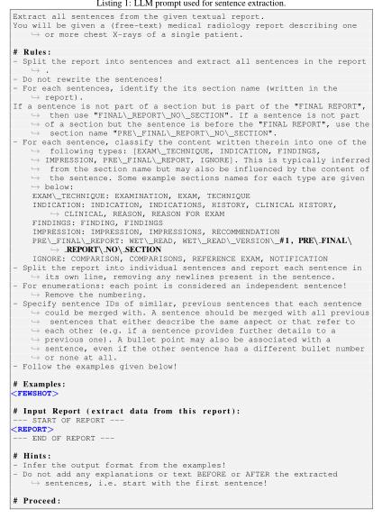
Listing 2: Few-shot example for sentence extraction.
Extracting the Observations In this step, we consider each sentence cluster (as identified during sentence extraction), in the FINDINGS and IMPRESSION sections. A sentence cluster contains one or more sentences that describe related aspects and may stretch over one of both of these sections. From each of these clusters, we now extract mentioned observations using the prompt shown in Listing 3 with few-shot examples similar to Listing 4. We apply this prompt to each sentence cluster individually and extract zero, one, or multiple observations each. The output is provided in the json-format and follows a similar structure as the final observation node, but we optimized it to be easy to fill by the LLM. The LLM is allowed to freely assign values to each of the json-fields. For name and summary sentence, we prompt the model to stay close to the original sentence, but it must remove any mentions of change and only keep the part relevant to the individual observation (if several observations are mentioned in one sentence). We successfully extracted observations from 227 266 studies (reports) while having parse errors for 360 studies.
Listing 3: LLM prompt used for observation extraction.
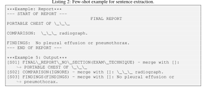
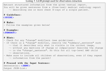
Listing 4: Few-shot example for observation extraction.
Extracting the Indication Next, we extract information about the INDICATION section and detect which FINDINGS or IMPRESSION sentences may provide information related to the indication. Therefore, the extracted INDICATION sentences and a list of all FINDINGS and IMPRESSION sentences are passed to the LLM using the prompt shown in Listing 5 with few-shot examples similar to Listing 6. The LLM predicts a json-structure containing several text fields for summaries of aspects in the indication, an answer for indication derived from the FINDINGS and IMPRESSION section, as well as relevant sentence IDs. We successfully extracted indictions from 227 596 studies (reports) while having parse errors for 30 studies.
Listing 5: LLM prompt used for indication extraction.
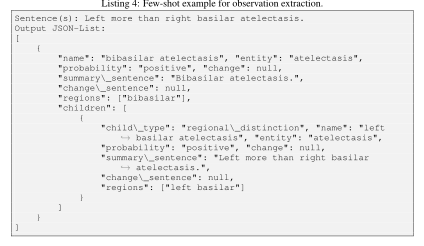
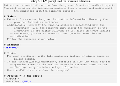
Listing 6: Few-shot example for indication extraction.
E.1.3 BUILDING SCENE GRAPHS
Entity Mapping We apply semantic entity mapping to modifiers (used to fill the attributes probability, certainty, positiveness, and modifiers), regions (attribute regions), finding entities (attribute obs entities), and changes (attribute changes).
For each of these we consider the associated tags extracted by the LLM during observation extraction and encode them into text embeddings using the BioLORD (Remy et al., 2024) model. We also encode all potential tags and their synonyms, defined for each type of tag in our reference definitions. Then we compute the cosine similarities of each tag with all reference tags of the same type. We pick the reference tag with the highest cosine similarity but threshold it at 0.5. If no reference tag was identified with cosine similarity ≥ 0.5, then we mark the tag as non-resolved. For finding entities, we follow a slightly more complicated matching approach. Instead of only considering the finding entity tags extracted by the LLM, we also consider pairs of these entities and extracted region tags as well as the extracted summary sentences and names for matching. We then try to match each of those with the reference finding tags and pick the ones with the highest cosine similarities.
The matched reference finding tags are stored in the obs entities attribute (non-resolved ones are kept in non resolved obs entities), matched reference regions are stored in the regions attribute, where we also store the distance as identified by the LLM (non-resolved regions are kept in non resolved regions). The matched changes are store in the changes attribute (non-resolved changes are discarded). For all modifiers, we use the modifier type defined for the matched reference tag. We matched all modifiers against all types of modifiers, which means that the modifier type identified by the LLM can be overwritten during matching. Finally, we extract the probability from the modifiers (this is a special modifier type), store it in the probability attribute and infer the certainty and positiveness attributes from it (using the reference definitions). The remaining modifiers are stored in the modifiers attribute (non-matched ones are discarded).
We additionally try to identify the laterality of the observations. Here, we do not use semantic entity mapping but rely on keywords instead. We consider the raw finding entities, regions, as well as the summary sentences, and search for any laterality-related mentions such as left, right, bilateral, and related terms. From this we infer the laterality and store it into the laterality attribute.
Reference Data and Standardization Using the reference definitions, we infer all obs_entities_parents, obs_categories, obs_subcategories, and default_regions from the matched obs_entities.

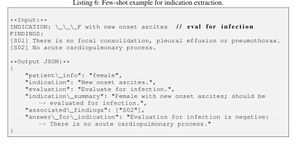
Next, we inspect the summary sentence and name attributes (extracted by the LLM) for underscores or mentions of changes. We track such issues (which are used for quality assessment) but do not apply any cleanup. Similarly, we check the change sentence for underscores and assert that it contains mentions of changes.
We further inspect the structure of observations and their children. If an observation mentions multiple different findings and has one child for each of these findings, then we lift these children to the top-level and discard the parent. Similarly, we merge multiple duplicate observations into one.
Finally, we try to resolve missing regions or improve their precision. If no regions could be extracted, we rely on the default regions derived from the obs entities instead, but consider the identified laterality. We also check whether these default regions are more precise than extracted ones. Then we check whether any identified region contradicts the identified laterality and remove them. We then either split or merge bilateral versions of the same region.
Graph Construction Based on the matched regions, we associate bounding boxes with the observations if available. Additionally, we build a tree of all mentioned regions and fill missing intermediate regions based on the reference data. This allows us to build a graph of region nodes relevant to the study.
We construct region_region_relations based on the reference data alone. located_at_relations are constructed based on the regions attribute of observations (direct_specified). Additionally, we infer located_at_relations relations for sub regions (sub_region) and bilateral versions of regions (bilateral). obs_relations are constructed based on the parent-child structure of observations and their child_type, as predicted by the LLM. obs_sent_relations are constructed based on the sentences each observation was derived from.
Finally, we attach the indication information extracted from the report. Therefore, we build an additional observation node based on the LLM-extracted answer for indication and the LLM-extracted associated sentences, from which we can infer the associated observations and can infer all relevant tags.
E.2 QUESTION-ANSWER GENERATION
E.2.1 TEMPLATE ENGINE
To construct QA-pairs, we develop a template-engine that considers the information in the scene graphs to construct the answers. The template engine generates a QA-pair by running the following steps:
- Filter observations and studies based on the template configuration, e.g. only keeping observations of specific sub-categories.
- Run a QA-strategy (indication, study abnormality, region abnormality, or finding) on the remaining scene graph. The strategy provides multiple named subsets of observations, variables to fill the template, as well as an overall state consisting of multiple tags (e.g. is the study positive, are there any devices,... ).
- Construct the template-based main answer by selecting and filling the answer-template based on the state returned by the QA-strategy and the returned variables. Tags and bounding boxes can be inferred from defined observation subsets. (Not all templates provide such main answers)
- Pick observation subsets identified by the QA-strategy and convert the observations into answer parts. The template configuration defines which subsets are picked and how they are ordered. Additionally, template-based prefix- or fallback-answers can be defined for each subset. Some subsets can also be excluded based on the QA-strategy state. These answers can be main-answers, details, or related information as defined in the configuration.
Additionally, the template engine supports variables, i.e. each template can be used to generate multiple QA-pairs. Variables can either be defined as lists (configured in the template) or can be
provided by the QA-strategy (which might infer variables from the current scene graph, e.g. all mentioned regions). The question may then also contain such template variables.
E.2.2 STRATEGIES AND TEMPLATES
Indication In this strategy, we use the extracted indication (if available) as the question. More precisely, we use the indication summary attribute from the indication node as the question text. The main-answer is constructed from the indication observation (i.e. the answer to the indication based on the finding sentences), while detail answer parts are constructed based on all associated finding observations. We include this question, if an indication observation is present in the scene graph.
Study abnormality In this strategy, we generate questions about abnormalities. This includes descriptions of the full study or specific categories of observations (e.g. devices), description of only abnormal findings, and yes/no questions of whether there are positive findings (overall or of specific categories) present in the study. We use the templates defined in Tab. 13.
The strategy identifies five types of observations: (i) finding (positive), (ii) finding (negative), (iii) device (positive), (iv) device (negative), (v) acquisition. Based on the specific template, these are selected as main-answers, details, or related information. Additionally, a template answer can be included, which is selected based on whether the study is abnormal or not. Some templates use different subcategories as variables, i.e. one question is generated for each of the defined subcategories, where observations are filtered based on this subcategory.
| Template (ID) | Question Example | Variables | Main answer | Details | Related Inf. |
|---|---|---|---|---|---|
| B01 describe all | Describe the given study. | – | finding (positive) device (positive) device (negative) finding (negative) acquisition | – | – |
| B02 describe abnormal | Describe all abnormal findings in the given study. | – | finding (positive) | – | device (positive) |
| B03 is abnormal | Are there any abnormal findings? | – | template finding (positive) | finding (negative) | device (positive) finding (negative) |
| B04 is normal | Is the study normal? | – | template | finding (positive) finding (negative) | finding (negative) device (positive) |
| B08 describe subcat | Evaluate the cardiac structures. | subcategory | finding (positive) finding (negative) | – | – |
| B09 describe abnormal subcat | Describe any pulmonary diseases and disorders suggested by the study. | subcategory | finding (positive) | – | – |
| B10 is abnormal subcat | Are there any fractures or bone diseases apparent from the study? | subcategory | template finding (positive) | finding (negative) | finding (negative) |
| B11 is normal subcat | Are the mediastinal and hilar contours normal? | subcategory | template finding (positive) | finding (negative) | finding (negative) |
| B12 describe device | Check the presence and position of devices, tubes, lines, and other foreign objects. | subcategory | device (positive) device (negative) | – | – |
| B13 has devices | Are there any signs of prior surgical procedures? | subcategory | template device (positive) | device (negative) | device (negative) |
| B14 describe acquisition | Assess the image quality and describe aspects related to image acquisition. | – | acquisition | – | – |
| B15 describe imaging artifacts | Describe any apparent imaging artifacts and imaging-related shadows. | – | acquisition | – | – |
| B16 has imaging artifacts | Are there any imaging artifacts or imaging-related shadows? | – | template acquisition | – | – |
Region abnormality In this strategy, we generate question about anatomical regions. This includes describing regions, answering yes/no questions about the abnormality of regions, or describing specific aspects of regions (e.g. devices). We use the templates defined in Tab. 14.
For a given region, the strategy first identifies observations associated with that region and classifies them into the five types defined in the study abnormality strategy. Additionally, it identifies observations in related regions. This includes positive findings in parent regions or the opposite laterality. Additionally, a template answer can be included, which is selected based on whether the region is abnormal or not.
Before generating QA-pairs, the strategy first identifies a set of regions. For each of these regions an individual QA-pair is generated. The set of regions is computed as follows: We always include a set of pre-defined default regions (the lungs, the heart,...) and include all regions explicitly mentioned in observations, as well as their parent regions. Additionally, we randomly sample regions. Their sampling probabilities are computed based on how often they are associated with positive vs. negative findings, i.e. the more often a region is associated with positive findings and the less often it is associated with negative findings, the more often we sample it as a question. This assures that we generate additional negative questions for regions that are only/mostly mentioned with positive findings.
| Template (ID) | Question Example | Variables | Main answer | Details | Related Inf. |
|---|---|---|---|---|---|
| C01 describe region | Describe the left lung. | region | finding (positive) device (positive) finding (negative) device (negative) | – | related regions |
| C02 describe abnormal region | Describe all abnormal findings in the lung bases. | region | finding (positive) | – | device (positive) related regions |
| C03 is abnormal region | Are there any abnormal findings in the mediastinum? | region | template finding (positive) | device (positive) finding (negative) | related regions |
| C04 is normal region | Is the heart normal? | region | template finding (positive) | region (positive) | finding (negative) related regions |
| C07 describe region device | Check the right chest for implants. | region subcategory | device (positive) device (negative) | – | related regions |
| C08 has region device | Are there any tubes, lines, or ports in or near the left lung? | region subcategory | template device (positive) | device (negative) | device (negative) related regions |
Finding In this strategy, we generate question about specific findings (radiological findings, diseaes, devices,... ). This includes descriptions of findings, yes/no questions about the presence of findings, location of findings, and severity of findings. We use the templates defined in Tab. 15.
For a given finding/device entity, the strategy first identifies observations associated with it and classifies them into the five types defined in the study abnormality strategy. Additionally, it identifies observations that contain related finding/device entities. This includes parent findings (i.e. findings that are parents of the current one), same subcat findings (i.e. findings having the same sub-category), correlated findings (based on statistics computed over the whole scene graph dataset), indications of the current finding, and findings that are indicative of the current finding. The observation subset can be selected based on the template configuration. Additionally, a template answer can be included, which is selected based on whether the finding is present or not and based on severity levels. This template may also be filled with information about the localization of the finding.
Before generating QA-pairs, the strategy first identifies a set of finding/device entities. For each of these entities an individual QA-pair is generated. The set of entities is computed as follows: We always include a set of pre-defined default entities and include all entities explicitly mentioned in observations, as well as their parent entities. Additionally, we randomly sample entities. Their sampling probabilities are computed based on how often they are mentioned positively vs. negatively (over all scene graphs), i.e. the more often a finding is mentioned positively and the less often it is mentioned negatively, the more often we sample it as a question. This assures that we generate additional negative questions for findings that are only/mostly mentioned positively.
| Template (ID) | Question Example | Variables | Main answer | Details | Related Inf. |
|---|---|---|---|---|---|
| D01 describe finding | Describe the pleural effusion. | finding | finding (positive) finding (negative) | – | parent findings indications indicative of same subcat correlated |
| D02 has finding | Is there any indication of pneumonia? | finding | template | finding (positive) finding (negative) | parent findings indications same subcat correlated |
| D03 where is finding | Where is the lung nodule located? | finding | template | finding (positive) finding (negative) | parent findings indications |
| D04 how severe is finding | How severe is the cardiomegaly? | finding | template | finding (positive) finding (negative) | parent findings indications |
| D05 describe device | Describe the endotracheal tube. | device | device (positive) device (negative) | – | parent findings same subcat |
| D06 has device | Is a pacemaker visible in the study? | device | template | device (positive) device (negative) | same subcat |
| D07 where is device | Where are the surgical clips located? | device | template | device (positive) device (negative) | same subcat |
E.3 QUALITY ASSESSMENT
Scene Graph Quality The scene graph quality aspects are computed by simply inspecting the observations nodes and checking which fields are set or empty. Additionally, we track issues during the graph construction procedure and derive quality aspects from them.
QA Quality We automatically assess the quality of the textual content of QA-pairs using Llama 3.1 8B (Grattafiori et al., 2024) as a judge for the five criteria presented in Tab. 12.
For rating entailment (Listing 7), we condition the model on the report, the question, as well as the answer parts and we rate each answer part individually.
Listing 7: LLM prompt used for entailment evaluation of generated answers.
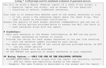
For rating relevance (Listing 8), we condition the model on the question as well as the answer parts (but not on the report) and we rate each answer part individually.
Listing 8: LLM prompt used for relevance evaluation of generated answers.
For rating completeness (Listing 9), we condition the model on the report, the question, as well as the full answer and we rate the full answer as a whole.
Listing 9: LLM prompt used for completeness evaluation of generated answers.

Rating (your task):
For rating question clarity (Listing 10), we condition the model on the question only and rate it.
Listing 10: LLM prompt used for question clarity evaluation of generated questions.
For rating answer clarity (Listing 11), we condition the answer parts only (but not on the report or question) and we rate each answer part individually.
Listing 11: LLM prompt used for answer clarity evaluation of generated answers.
You will be given a medical Answer to an unknown question about a → radiological chest X-ray study (which is not provided).
E.4 RESOURCES FOR DATASET CONSTRUCTION AND EVALUATION
E.4.1 SOURCE DATASETS
MIMIC-CXR (Johnson et al., 2024b; 2019a; Goldberger et al., 2000) We use the MIMIC-CXR dataset version 2.1.0 (https://physionet.org/content/mimic-cxr/2.1.0/ as the source of radiology reports from which we extract the scene graphs. It contains 227 835 radiographic (chest X-ray) studies performed at the Beth Israel Deaconess Medical Center in Boston, MA, USA. It is licensed under the PhysioNet Credentialed Health Data License 1.5.0.
MIMIC-CXR-JPG (Johnson et al., 2024a; 2019b; Goldberger et al., 2000) We use the MIMIC-CXR-JPG dataset version 2.1.0 (https://physionet.org/content/mimic-cxr-jpg/
2.1.0/) as the source of images for localization (the CXAS segmntation model is applied on these images). Additionally, we use the provided radiologist annotations (mimic-cxr-2.1.0-test-set-labeled.csv) as targets to evaluate the quality of extracted finding tags (Tabs. 2a and 7). The dataset is derived from MIMIC-CXR and is licensed under the PhysioNet Credentialed Health Data License 1.5.0.
Chest ImaGenome (Wu et al., 2021a;b; Goldberger et al., 2000) We use the Chest ImaGenome Dataset version 1.0.0 (https://physionet.org/content/chest-imagenome/1.0. 0/) as a source of anatomical region bounding boxes for localization. Additionally, we use their provided scene graphs as a baseline for the evaluations of our scene graphs (Tabs. 2 and 7 to 10). It contains scene graphs for 242 072 frontal images from MIMIC-CXR that have been created using rule-based natural language processing and CXR atlas-based bounding box detection. The dataset is derived from MIMIC-CXR and is licensed under the PhysioNet Credentialed Health Data License 1.5.0.
CXR-LT 2024 (Holste et al., 2025; 2024; Goldberger et al., 2000) We use the CXR-LT 2024 dataset version 2.0.0 (https://physionet.org/content/cxr-lt-iccv-workshop-cvamd/2.0.0/) as targets to evaluate the quality of extracted finding tags (Tabs. 2a and 8). More precisely, we use the gold standard dataset provided for Task 2 in the CXR-LT 2024 challenge tasks (406 reports, 26 classes). The dataset is derived from a small subset of MIMIC-CXR and was hand-labeled by radiologists. It is licensed under the PhysioNet Credentialed Health Data License 1.5.0.
MS-CXR (Boecking et al., 2024; 2022; Goldberger et al., 2000) We use the MS-CXR dataset version 1.1.0 (https://physionet.org/content/ms-cxr/1.1.0/) as targets to evaluate the quality of extracted finding boxes (Tabs. 2b and 9). The dataset contains 1162 image-sentence pairs of bounding boxes and corresponding phrases (and their finding classes) for 8 different findings. It is derived from a small subset of MIMIC-CXR and was hand-labeled by radiologists. It is licensed under the PhysioNet Credentialed Health Data License 1.5.0.
REFLACX (Bigolin Lanfredi et al., 2021; 2022; Goldberger et al., 2000) We use the REFLACX dataset version 1.0.0 (https://physionet.org/content/reflacx-xray-localization/1.0.0/) as targets to evaluate the quality of extracted finding boxes (Tabs. 2b and 10). The dataset provides eye-tracking data collected for 3032 frontal chest x-rays from the MIMIC-CXR dataset. Additionally, it provides hand-labeled ellipses localizing for several anomalies present in the images. We only use the ellipses but do not use the eye-tracking data. It is licensed under the PhysioNet Credentialed Health Data License 1.5.0.
E.4.2 MODELS
LLM Selection We choose the information extraction model (Llama 3.1 70B) based on the following criteria:
- Open weights and locally hostable (required due to the MIMIC dataset licenses).
- Fast and efficient to run on large amounts of data.
- Sufficient extraction quality and instruction following. Sophisticated reasoning capabilities are not required.
- No vision component is required.
While using other models would be possible, we choose Llama 3.1 70B based on preliminary experiments (at the start of dataset construction). Those experiments indicated that it provides good trade-offs for the points above.
The study of alternative models may be interesting. However, we do not expect major improvements in data quality, as our semantic entity mapping and our automatic quality assessment already provide a robust framework to assure data quality even with small data extraction errors. Therefore, we leave this to future work.
Llama 3.1 70B (Grattafiori et al., 2024) We use the AWQ-INT4 (Lin et al., 2024) quantized version of Llama 3.1 70B Instruct provided by the Huggingface hub at https://huggingface.co/hugging-quants/Meta-Llama-3.1-70B-Instruct-AWQ-INT4. The model is derived from the https://huggingface.co/meta-llama/Llama-3.1-70B-Instruct and is licensed under the LLAMA 3.1 COMMUNITY LICENSE AGREEMENT. We limit the maximum number of tokens to 6144.
Llama 3.1 8B (Grattafiori et al., 2024) We use the AWQ-INT4 (Lin et al., 2024) quantized version of Llama 3.1 70B provided by the Huggingface hub at https://huggingface.co/hugging-quants/Meta-Llama-3.1-8B-Instruct-AWQ-INT4. The model is derived from the https://huggingface.co/meta-llama/Llama-3.1-8B-Instruct and is licensed under the LLAMA 3.1 COMMUNITY LICENSE AGREEMENT. We limit the maximum number of tokens to 8192.
CXAS (Seibold et al., 2022; 2023) We use the model provided by the CXAS Python See also https://github.com/library https://pypi.org/project/cxas/. ConstantinSeibold/ChestXRayAnatomySegmentation. It is licensed under the Attribution-NonCommercial-ShareAlike 4.0 International license. We run segmentation of all anatomical structures on half the original image resolution (half original image width and height).
BioLORD (Remy et al., 2024) We use the BioLORD-2023-C variant provided by the Hug-gingface model hub at https://huggingface.co/FremyCompany/BioLORD-2023-C and licensed under the MIT license. To apply the model, we use the Sentence Transformers library (https://github.com/UKPLab/sentence-transformers), which is licensed under the Apache-2.0 license.
Model Inference Details For all LLM-based information extraction steps, we rely on the vLLM library (Kwon et al., 2023) (https://github.com/vllm-project/vllm, Apache-2.0 license) for inference. We run all models with temperature = 0.0. All json-outputs are parsed using the Pydantic libary (https://docs.pydantic.dev).
E.4.3 COMPUTATIONAL COSTS
Each dataset construction step can run on an individual Nvidia A100 GPU, but we use multiple GPUs in parallel, with each GPU responsible for a different subset of the dataset. Semantic segmentation of all 158 anatomical structures using the CXAS models takes about 6 seconds per image, leading to a total of about 628 GPU hours. Sentence extraction takes about 1 second per study (report), leading to a total of about 65 GPU hours (for 227 835 studies). Observation extraction takes about 1.7 seconds per study, leading to a total of about 108 GPU hours. Indication extraction takes about 0.3 seconds per study, leading to a total of about 19 GPU hours. Scene graph construction (including entity matching) takes about 0.6 seconds per study, leading to a tool of about 38 hours. Question-answer generation does not require a GPU but takes about 9 seconds per study (including all question templates and strategies), leading to a total of about 24 days. However, multiple processes can be run in parallel on a single machine, leading to an effective time of only about a day for all 42M QA-pairs. Quality assessment of QA texts again requires a GPU and consists of 5 individual steps that can be run in parallel. Overall the assessment takes about 6 GPU days for all 42M QA-pairs.
Societal Impact As a large vision-language dataset for medical imaging, this dataset has significant potential for societal impact. However, its use as a training source for models employed in clinical or medical applications also poses a substantial risk of misdiagnosis, highlighting the need for caution. Therefore, we strongly advise against relying solely on this dataset for fine-tuning or evaluating such models. On the other hand, this dataset can facilitate the development of large and interactive VQA models, which can provide supplemental information for patients, serve as a training tool for healthcare professionals, or optimize clinical workflows. The provided annotations, including bounding boxes and tags, further enhance its utility by providing a level of transparency and explainability in model predictions, allowing for more informed interpretation and analysis. By sparking research in this direction, this dataset can contribute to the advancement of the field and ultimately lead to positive long-term societal impacts. Nevertheless, it is essential to approach this
dataset with caution, recognizing its limitations and potential risks if used improperly. As such, we consider this dataset a valuable research asset, but not yet suitable as a (sole) training source for real-world medical applications, emphasizing the need for careful evaluation and validation.
F STRUCTURED VQA TASK
F.1 FURTHER STRUCTURED VQA RESULTS
| Ours (ablations) | Ours (default) | Baselines | ||||||||||
|---|---|---|---|---|---|---|---|---|---|---|---|---|
| Group | Metric | Abl. 1 | Abl. 2 | Abl. 3 | Abl. 4 | Abl. 5 | PT(1M) | PT(2M) | PT→FT | MAIRA-2 | Qwen3-VL | LLaVA-Med 1.5 |
| Setup | CXR-QBA Set | FT(1M) | FT(1M) | FT(1M) | FT(1M) | FT(1M) | PT(1M) | PT(2M) | PT(1M)→FT(1M) | ✗ | ✗ | ✗ |
| Setup | Boxes | ✗ | ✓ | ✓ | ✓ | ✓ | ✓ | ✓ | ✓ | ✓ | ✓ | ✓ |
| Setup | Tags | ✗ | ✗ | ✗ | ✓ | ✓ | ✓ | ✓ | ✓ | ✗ | ✗ | ✗ |
| Setup | Box/Tag Position | – | after text | before text | after text | before text | after text | after text | after text | after text | after text | after text |
| RadFact* | Logical Prec. | 0.75 | 0.76 | 0.76 | 0.76 | 0.76 | 0.67 | 0.68 | 0.78 | 0.25 | 0.63 | 0.47 |
| RadFact* | Logical Rec. | 0.74 | 0.75 | 0.75 | 0.75 | 0.75 | 0.69 | 0.70 | 0.77 | 0.64 | 0.58 | 0.08 |
| RadFact* | Logical F1 | 0.74 | 0.74 | 0.75 | 0.75 | 0.75 | 0.70 | 0.71 | 0.77 | 0.27 | 0.57 | 0.34 |
| RadFact* | Grounding Prec. | – | 0.88 | 0.87 | 0.88 | 0.87 | 0.87 | 0.88 | 0.89 | 0.69 | 0.61 | – |
| RadFact* | Grounding Rec. | – | 0.88 | 0.90 | 0.88 | 0.89 | 0.92 | 0.92 | 0.90 | 0.12 | 0.51 | – |
| RadFact* | Grounding F1 | – | 0.83 | 0.83 | 0.83 | 0.83 | 0.85 | 0.86 | 0.85 | 0.32 | 0.37 | – |
| RadFact* | Spatial Prec. | – | 0.68 | 0.67 | 0.68 | 0.67 | 0.60 | 0.61 | 0.70 | 0.12 | 0.40 | – |
| RadFact* | Spatial Rec. | – | 0.67 | 0.68 | 0.68 | 0.68 | 0.64 | 0.65 | 0.70 | 0.07 | 0.31 | – |
| RadFact* | Spatial F1 | – | 0.63 | 0.63 | 0.64 | 0.63 | 0.60 | 0.62 | 0.67 | 0.06 | 0.23 | – |
| RadStrucVQA (Tags) | Finding Prec. | – | – | – | 0.68 | 0.68 | 0.67 | 0.68 | 0.70 | – | – | – |
| RadStrucVQA (Tags) | Finding Rec. | – | – | – | 0.67 | 0.66 | 0.61 | 0.62 | 0.68 | – | – | – |
| RadStrucVQA (Tags) | Finding F1 | – | – | – | 0.68 | 0.67 | 0.68 | 0.69 | 0.70 | – | – | – |
| RadStrucVQA (Tags) | Finding-pos Prec. | – | – | – | 0.40 | 0.41 | 0.32 | 0.37 | 0.45 | – | – | – |
| RadStrucVQA (Tags) | Finding-pos Rec. | – | – | – | 0.29 | 0.26 | 0.13 | 0.16 | 0.31 | – | – | – |
| RadStrucVQA (Tags) | Finding-pos F1 | – | – | – | 0.39 | 0.39 | 0.36 | 0.40 | 0.43 | – | – | – |
| RadStrucVQA (Tags) | Region Prec. | – | – | – | 0.67 | 0.67 | 0.61 | 0.61 | 0.69 | – | – | – |
| RadStrucVQA (Tags) | Region Rec. | – | – | – | 0.66 | 0.66 | 0.62 | 0.63 | 0.68 | – | – | – |
| RadStrucVQA (Tags) | Region F1 | – | – | – | 0.66 | 0.67 | 0.64 | 0.65 | 0.69 | – | – | – |
| RadStrucVQA (Tags) | Region-pos Prec. | – | – | – | 0.29 | 0.34 | 0.24 | 0.26 | 0.37 | – | – | – |
| RadStrucVQA (Tags) | Region-pos Rec. | – | – | – | 0.21 | 0.21 | 0.10 | 0.12 | 0.25 | – | – | – |
| RadStrucVQA (Tags) | Region-pos F1 | – | – | – | 0.29 | 0.32 | 0.27 | 0.30 | 0.36 | – | – | – |
| RadStrucVQA (Tags) | Main-category Prec. | – | – | – | 0.73 | 0.73 | 0.66 | 0.67 | 0.75 | – | – | – |
| RadStrucVQA (Tags) | Main-category Rec. | – | – | – | 0.70 | 0.70 | 0.63 | 0.64 | 0.72 | – | – | – |
| RadStrucVQA (Tags) | Main-category F1 | – | – | – | 0.72 | 0.72 | 0.68 | 0.70 | 0.74 | – | – | – |
| RadStrucVQA (Tags) | Main-category-pos Prec. | – | – | – | 0.49 | 0.52 | 0.39 | 0.43 | 0.55 | – | – | – |
| RadStrucVQA (Tags) | Main-category-pos Rec. | – | – | – | 0.36 | 0.34 | 0.16 | 0.19 | 0.38 | – | – | – |
| RadStrucVQA (Tags) | Main-category-pos F1 | – | – | – | 0.47 | 0.49 | 0.42 | 0.45 | 0.52 | – | – | – |
| RadStrucVQA (Tags) | Sub-category Prec. | – | – | – | 0.71 | 0.71 | 0.69 | 0.70 | 0.73 | – | – | – |
| RadStrucVQA (Tags) | Sub-category Rec. | – | – | – | 0.67 | 0.67 | 0.59 | 0.60 | 0.69 | – | – | – |
| RadStrucVQA (Tags) | Sub-category F1 | – | – | – | 0.69 | 0.69 | 0.69 | 0.70 | 0.71 | – | – | – |
| RadStrucVQA (Tags) | Sub-category-pos Prec. | – | – | – | 0.47 | 0.50 | 0.37 | 0.41 | 0.53 | – | – | – |
| RadStrucVQA (Tags) | Sub-category-pos Rec. | – | – | – | 0.34 | 0.32 | 0.15 | 0.18 | 0.36 | – | – | – |
| RadStrucVQA (Tags) | Sub-category-pos F1 | – | – | – | 0.45 | 0.46 | 0.40 | 0.43 | 0.49 | – | – | – |
| RadStrucVQA (Tags) | Bbox-pos-entity Prec. | – | – | – | 0.31 | 0.32 | 0.25 | 0.27 | 0.36 | – | – | – |
| RadStrucVQA (Tags) | Bbox-pos-entity Rec. | – | – | – | 0.22 | 0.20 | 0.11 | 0.13 | 0.25 | – | – | – |
| RadStrucVQA (Tags) | Bbox-pos-entity F1 | – | – | – | 0.26 | 0.26 | 0.26 | 0.28 | 0.32 | – | – | – |
F.2 RAD STRUC VQA METRIC
| Pearson Correlation | |||
|---|---|---|---|
| Metric | Llama 3.1 8B ↔ Llama 3.1 70B | Llama 3.1 8B ↔ Qwen3-32B | Llama 3.1 70B ↔ Qwen3 32B |
| Logical Prec. | 0.90 | 0.94 | 0.98 |
| Logical Rec. | 0.90 | 0.90 | 0.97 |
| Grounding Prec. | 0.97 | 0.99 | 0.99 |
| Grounding Rec. | 0.96 | 0.99 | 1.00 |
| Finding Prec. | 0.96 | 0.98 | 0.99 |
| Finding Rec. | 0.97 | 0.97 | 0.98 |
| Finding-pos Prec. | 0.88 | 0.92 | 0.96 |
| Finding-pos Rec. | 0.90 | 0.92 | 0.96 |
| Region Prec. | 0.97 | 0.98 | 0.98 |
| Region Rec. | 0.97 | 0.97 | 0.98 |
where ssub (H, C) ∈ [0, 1] is a sub-metric specific scoring function considering the hypothesis set H given the context set C. For precision H = Ŷ is the prediction set and C = Y is the target set, while for recall H = Y and C = Ŷ.
We compute C[h] by prompting an LLM to (i) identify entailment of h given all context elements in C, where h can be ENTAILED or NOT ENTAILED (neutral or contradicting); and (ii) provide the relevant evidence for entailment, i.e. the context units c ∈ C that support h. The LLM is given only the textual descriptions of each element (answer part), i.e. the entailment classification is purely logical and does not consider localization or any tags. Note that C[h] = {} if h is not entailed.
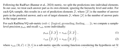
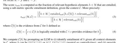

while the relevant subset of hypothesis elements is identified using the sub-metric specific
(6)
relevantsub (h) ∈ {true, false}.
The definitions for each sub-metric can be found in Tab. 18.
| Sub-metric | entailed_sub(h, C[h]) | relevant_sub(h) |
|---|---|---|
| logical | C[h] is not empty; i.e. there is positive evidence for h in C and h does not contradict C | always true |
| grounding | entailed_logical(h, C[h]) ∧ IoH(h, C[h]) ≥ 0.5; IoH is the intersection between boxes in h and boxes in C[h] over the total box area in h, using box masks (unions of boxes) | h has bounding boxes ∧ entailed_logical(h, C[h]) |
| spatial | entailed_grounding(h, C[h]) | h has bounding boxes |
| finding | entailed_logical(h, C[h]) ∧ each finding tag in h is present in any of C[h], considering only C[h] with the same positivity | h has finding tags |
| finding-pos | entailed_finding(h, C[h]) | relevant_finding(h) ∧ h is positive |
| region | entailed_logical(h, C[h]) ∧ each region tag in h is present in any of C[h], considering only C[h] with the same positivity | h has region tags |
| region-pos | entailed_region(h, C[h]) | relevant_region(h) ∧ h is positive |
| main-category | entailed_logical(h, C[h]) ∧ each finding main-category tag in h is present in any of C[h], considering only C[h] with the same positivity | h has finding main category tags |
| main-category-pos | entailed_main-category(h, C[h]) | relevant_main-category(h) ∧ h is positive |
| sub-category | entailed_logical(h, C[h]) ∧ each finding sub-category tag in h is present in any of C[h], considering only C[h] with the same positivity | h has finding sub category tags |
| sub-category-pos | entailed_sub-category(h, C[h]) | relevant_sub-category(h) ∧ h is positive |
| bbox-pos-entity | entailed_finding(h, C[h]) ∧ entailed_grounding(h, C[h]) | relevant_finding-pos(h) ∧ relevant_spatial(h) |
Implementation Details The final precision/recall scores are computed by averaging the sample-level scores. F1 scores can also be computed by first taking the per-sample harmonic mean of precision and recall before averaging the sample-level F1 scores. Invalid answers, samples with LLM parse errors during entailment computation, as well as samples without relevant hypotheses are ignored during averaging. We use the same entailment prompts and few-shot examples as in RadFact (Bannur et al., 2024) but use the Llama 3.1 8B (Grattafiori et al., 2024) model, allowing us to compute the metric locally.
F.3 EXPERIMENTAL SETUP
Vision-Language Model Training Our vision-language model follows the Llava architecture (Liu et al., 2023), using Rad-DINO (Pérez-Garcı́a et al., 2025) (microsoft/rad-dino) for image encoding and the 3B Llama 3.2 language model (https://huggingface.co/meta-llama/Llama-3.2-3B-Instruct) connected via an MLP projection layer. We freeze the image encoder and all existing language model parameters but add new special tokens (with trainable embeddings) and apply LoRA (Hu et al., 2021) to the language model. Therefore, we only train the projection layer, the LoRA parameters, and the newly added token embeddings (keeping the existing token embeddings frozen). We train for one epoch, either on 1M QA pairs randomly sampled from the fine-tuning (FT) grade set or on 1M QA pairs randomly sampled from the pre-training (PT) grade

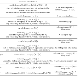
set of our CXR-QBA dataset (MIMIC-CXR’s train split). We use autoregressive training but only apply the loss to answer tokens. For image encoding and projection, we adopt the hyperparameters of MAIRA-2 (Bannur et al., 2024): We square-crop the images and resize them to 518 × 518, leading to 37 × 37 = 1369 image patches (i.e. image tokens), then we use the features of the last image encoder layer, and project the image tokens using 4 projection layers with GeLU activations. For LoRA, we use r = 64, α = 16, and dropout 0.05. The maximum number of tokens for the language model is restricted to 2048. We use the AdamW optimizer with cosine annealing scheduling with 500 warmup steps, maximum learning rate 1e − 3, no weight decay, a batch size of 4 with 16 accumulation steps, gradient norm clipping at 1.0, and bf16 precision. All models are evaluated on the test split (following MIMIC-CXR) of our CXR-QBA fine-tuning (FT) grade set.
Prompt and Special Tokens Our question prompt follows the template shown in Listing 12, where <boi> (begin of image), <eoi> (end of image), and <imgref1> (first image reference) are newly added special tokens, <img> tokens are replaced by image token features, and {QUESTION} is replaced by the specific question.
Consider the following chest X-ray image: <boi><imgref1><img>...<eoi> {
    → QUESTION}
The answers are formatted into sequences using XML-style structures and special tokens to represent tags and bounding boxes. An example is given in Listing 13.
<answer>
  <regions><bilateral><lungs></regions>
  <probability><certain><neg><probability>
  <categories>
    <ANATOMICAL_FINDING><DISEASE>
    <subcat>LUNG FIELD</subcat><subcat>PULMONARY DISEASES</subcat>
  </categories>
  <entities><entity>pneumothorax</entity></entities>
  <modifiers></modifiers>
  <box><imgref1><x51><y18><x90><y87><box>
  <box><imgref1><x09><y19><x52><y93></box>
  No, there is no indication of pneumothorax.
</answer>
We use special start and end tokens for answer parts (<answer> / </answer>), bounding boxes (<box> / </box>), and groups of tags (<regions> / </regions>, <probability> / </probability>, <categories> / </categories>, <entities> / </entities>, <modifiers> / </modifiers>). For some tags we use individual special tokens, namely for laterality (e.g. <bilateral>), regions (e.g. <lungs>), certainty (e.g. <certain>), positivity (e.g. <neg>), and main categories (e.g. <ANATOMICAL FINDING>). For others we use start/end tokens and normal text, namely for sub-categories (<subcat> / </subcat>) and finding entities (<entity> / </entity>). Bounding boxes are listed after all other tags, where we use <box> / </box> tokens and refer back to the image using <imgref1>. Inside the box-tokens we use special relative coordinate tokens (following MAIRA-2 (Bannur et al., 2024)) that represent the normalized (x1, y1, x2, y2) coordinates of the bounding box, each quantized to 100 different tokens per dimension. We use different tokens for the x- and y-dimensions but share them for both corners (e.g. x1 and x2 share the same token set). The textual description is the last part of each answer part and consists of plain text without special tokens. If an answer consists of multiple answer parts, then each answer part uses an individual block as in Listing 13. All new token embeddings are initialized close to the existing token embeddings, where we try to initialize them based on keywords defined for each token. More precisely, given a set of keywords for a new token, we tokenize the keywords using the old vocabulary and compute the average embedding of all these tokens. This is then used as the initialization for the new token.
MAIRA-2 Baseline We use the MIARA-2 (Bannur et al., 2024) checkpoint available at https: //huggingface.co/microsoft/maira-2. We freeze the full model but modify the prompt.
More precisely, we use their original prompt for grounded report generation but slightly modify it, asking the model to answer to the question (included in the modified prompt) instead of reporting all findings in the image. The rest of the prompt is kept unchanged. This model is then evaluated on the same test set as our vision-language model. It is capable of generating individual answer parts, each with bounding boxes, but does not generate bounding boxes for negative answers and cannot generate any tags.
Qwen3-VL We use the 4B Instruct version of Qwen3VL, using the checkpoint available at https://huggingface.co/Qwen/Qwen3-VL-4B-Instruct. We do not train the model but prepare a prompt that asks the model to provide individual answer sentences per finding and to provide textual bounding boxes. For this we also provide a reference size of the image, based on which we evaluate the predicted bounding boxes. All image processing follows their implementation.
Llava-Med v1.5 We use the checkpoint provided at https://huggingface.co/chaoyinshe/llava-med-v1.5-mistral-7b-hf, such that the huggingface library can directly be used for inference. We do not train the model and use the same prompts as for Qwen-VL. All image processing follows their implementation.